

Abstract
Various elements of the Earth system have the potential to undergo critical transitions to a radically different state, under sustained changes to climate forcing. The Atlantic meridional overturning circulation (AMOC) is of particular importance for North Atlantic heat transport and is thought to be potentially at risk of passing such a tipping point (TP). In climate models, the location and likelihood of such TPs depends on model parameters that may be poorly known. Reducing this parametric uncertainty is important to understand the likelihood of tipping behaviour. In this letter, we develop estimates for parametric uncertainty in a simple model of AMOC tipping, using a Bayesian inversion technique. When applied using synthetic ('perfect model') salinity timeseries data, the technique drastically reduces the uncertainty in model parameters, compared to prior estimates derived from previous literature, resulting in tighter constraints on the AMOC TPs. To visualise the impact of parametric uncertainty on TPs, we extend classical tipping diagrams by showing probabilistic bifurcation curves according to the inferred distribution of the model parameter, allowing the uncertain locations of TPs along the probabilistic bifurcation curves to be highlighted. Our results show that suitable palaeo-proxy timeseries may contain enough information to assess the likely position of AMOC (and potentially other Earth system) TPs, even in cases where no tipping occurred during the period of the proxy data.
Export citation and abstract BibTeX RIS

Original content from this work may be used under the terms of the Creative Commons Attribution 4.0 license. Any further distribution of this work must maintain attribution to the author(s) and the title of the work, journal citation and DOI.
1. Introduction
Several elements of the Earth system have been identified as at risk of crossing a tipping point (TP) [1] in which the element loses stability and passes from its current stable state to a new, possibly quite different, stable state. A well-studied example is the Atlantic meridional overturning circulation (AMOC), a system of ocean currents that influences Northern Hemisphere climate by transporting heat from the tropics to the higher latitude North Atlantic, but which at times in the distant past may have 'switched off' via such a tipping process [1, 2]. Such a switch-off would be expected to cause widespread cooling and drying over the northern hemisphere, major changes to tropical rainfall systems and mid-latitude jets, and regional sea level rise (e.g. [3]). In order to build societal resilience to future climate changes, it is important to determine whether such tipping could happen in the present or future states of the climate system. Given our incomplete knowledge of the real world, the answer to this question will necessarily be probabilistic.
Tipping behaviour in the climate system has often been studied using low order models (e.g. [4–6]). Such models often show tipping behaviour when some system parameter (e.g. the strength of some climate forcing factor) passes a critical value. There is a well-developed mathematical theory of these bifurcations [7–10], which can be used to analyse the response to changes in climate forcing. Insights from low order models have been shown to be relevant to tipping behaviour seen in far more complex climate general circulation models (GCMs) [6].
In classical bifurcation theory, model parameters are assumed known. However, in practical climate modelling, parameter values are uncertain and often have to be estimated indirectly. We can think of a climate model as consisting of a parameter-dependent system of ordinary differential equations (ODEs):
where vector x represents the climate state and vector r of dimension d represents the d model parameters. The uncertainty in parameter values can be represented by passing from the deterministic ODE system (1) to a system of random ODEs:

where  is a random vector corresponding to sampling of d uncertain model parameters from a probability space. Hence, we have to deal with parametric uncertainty, i.e. uncertainty about the values of some model inputs (see e.g. [11]). For practical modelling of TPs in climate systems this leads to two key questions:
- Q1:How can the probability distribution of the model parameters be inferred?
- Q2:How does this parametric uncertainty affect model estimates of the tipping behaviour of the system?
Q1 is a generic question for climate modelling, on which there has been much research. Many approaches to parameter estimation have been investigated [12–15]. The use of Bayesian inference methods [13] has become widely used in climate science (see e.g. [16, 17]), and forms the basis of many climate change assessments using state-of-the art climate models (e.g. [18–20]). Typically, available physical constraints are combined with an element of expert opinion to provide an initial (prior) distribution for the parameters in question. This prior distribution is then modified by evaluating the ability of the model to simulate a range of observed properties of the climate system, under different choices of parameters. Parameter settings that produce good simulations of the target observations are assigned a higher weight, resulting in a modified (posterior) parameter distribution. The approach can be considered as a problem in inverse modelling or data assimilation.
In contrast, Q2 has received much less attention, despite a few exploratory studies (e.g. [6, 16, 21–23]). The link between model parameter uncertainty and TPs is important, as an apparently small uncertainty in a parameter may lead to a large uncertainty in the location of TPs or the shape of the bifurcation curve. Hence, a TP might be much closer to the current system state than expected from the 'best estimate' model parameters [24]. Only recently, this link between parametric uncertainty and bifurcations has emerged as a sub-area within the theory of nonlinear dynamics [25–28], with methods being developed for applications in fields including aerospace engineering [29, 30] and biomedical science [31]. Studies in the climate domain have been limited; however [16, 21, 22] show the possibility of AMOC collapse in certain parameter regimes of simple and intermediate-complexity climate models.
Here, we address the link between parametric uncertainty and tipping dynamics, by showing that a Bayesian approach to parameter estimation can produce refined knowledge of the position of TPs, even if the observations used for the Bayesian constraints are sampled well away from any TPs (e.g. using recent AMOC observations, sampled during a period of strong AMOC, to constrain potential future AMOC tipping). We go on to present some visual tools to aid interpretation of the resulting probabilistic estimates of the tipping behaviour, including probabilistic visualisations of the classical bifurcation diagram, and of how far the system may be from tipping. We illustrate our approach using a widely-studied, low-order model of AMOC tipping. While our purpose here is primarily to use this simple model to present the method and the visualisation tools, we discuss in the final section how our ideas may be applicable to more complex models and 'real world' estimation of risks of climate tipping.
The framework is sketched in figure 1. We use the Stommel–Cessi model for the AMOC to illustrate our method [5]. Note that this bypasses the step of model selection that is an important part of some Bayesian approaches [32]. We discuss the importance of this step in the final section of this paper. Our approach is not limited to this particular model.

Figure 1. Outline of the steps described in this paper. Given a climate model, we provide prior ranges for uncertain model parameters and present a Bayesian inference method to derive corresponding parameter probability distributions. For visualisation, we construct corresponding probabilistic tipping diagrams.
Download figure:
Standard image High-resolution imageSection 2 outlines the AMOC box model [5] and its deterministic tipping behaviour. We present physically-constrained prior ranges for model parameters, and a Bayesian inference method to infer probability distributions based on these physical constraints and available data. The derived probability distribution for the parameters implies a probabilistic view of the TPs, and in section 3, we construct corresponding probabilistic tipping diagrams to illustrate how the parametric uncertainty leads to uncertainty in tipping behaviour. We conclude with a discussion of the implications of our work for robust estimation of the risk of crossing an AMOC TP, and potentially other Earth System TPs.
2. Problem setup
To illustrate our method, we consider here the Stommel–Cessi box model [5], which is a simplified description of the AMOC based on two boxes, an equatorial (e) and a polar (p) one. Temperature differences  and salinity differences
  may arise due to an atmospheric freshwater flux p(t) leading to a density gradient, in turn enabling a circulation between the boxes.
As described in [33, section 6.2.1], the system can be reduced to an attracting invariant manifold and after rescaling one obtains the reduced dynamics as:
with  corresponding to a dimensionless salinity difference, where αS
and αT
are saline contraction and thermal expansion coefficients and θ is a reference value for
corresponding to a dimensionless salinity difference, where αS
and αT
are saline contraction and thermal expansion coefficients and θ is a reference value for  . For a physical interpretation, note that in this model x is typically positive (subtropics saltier than subpolar), meaning that salinity is acting to slow the AMOC, while the temperature difference is acting to drive it. Thus small x corresponds to the current strong AMOC state, while large x corresponds to weak or reversed AMOC. The parameter µ is proportional to the atmospheric freshwater flux, and the parameter:

is the ratio of the diffusive timescale td (representing wind-driven transports) to the advective timescale due to the AMOC itself, ta . The steady states of (3) are given by:
The precise shape of the equilibrium curve for x as a function of µ depends crucially on the parameter η2. Although, for all η2, the points  and
and  are equilibria, the dynamics show important qualitative differences for different values of η2. In particular, on
  (red solid line in figure 2) there is a cusp bifurcation point at µ = 1.
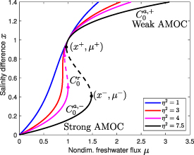
Figure 2. The shape of the equilibrium curve (5) depends crucially on the value of the parameter η2. For  , there are no TPs whereas for
  , the curve is S-shape and admits two fold points (magenta and black dots).
Download figure:
Standard image High-resolution imageParameter regime η 2 > 3 (weak diffusion): In this case, the steady states (5) form the classical S-shape (figure 2). There are two fold bifurcations linked to variation in the bifurcation parameter µ with corresponding fold points:
where  . The TPs
  and
and  split the curve into an upper and lower attracting branch of fixed points
  and
and  (upper and lower solid magenta and black lines in figure 2). The upper branch (
 ) corresponds to a stable weak AMOC, while the lower branch (
 ) corresponds to a stable strong AMOC. For values of µ between µ− and
  both strong and weak AMOC states are stable. The two attracting branches are connected by a repelling branch (unstable equilibrium)
  (dashed magenta and black lines in figure 2). Tipping of the AMOC from its current strong stable state to a new weak stable state might occur if the fresh water flux µ were increased beyond µ−. The bistable regime leads to a hysteresis behaviour of the AMOC, in which reversing the bifurcation parameter µ to its value before the tipping occurred would not be enough to switch the AMOC back to its strong state. The freshwater flux would have to be further decreased below
  to get the strong stable state back again.
Parameter regime η 2 > 3 (strong diffusion): In this case, there are no longer any values of µ that give bistability of the system, and no bifurcations on varying µ.
The true value of η2 is unknown. Figure 2 reveals that its value makes a major difference in the shape of the equilibrium curve (5). A mis-specification of the value of η2 can crucially change the overall qualitative behaviour of (3). Therefore, a quantification of the effect of the uncertainty in η2 is needed. In the rest of this section we describe an approach to constrain the value of η2. First (section 2.1), we determine a prior parameter range for η2 based on physical constraints and previous evidence. Then (section 2.2), we infer a probability distribution of the parameter η2 using a Bayesian inference technique. Since the freshwater flux µ is the main forcing parameter and is modified by climate change, we leave it as a deterministic bifurcation parameter here.
2.1. Prior physical constraints on model parameters
Different values for η2 are used in the literature (e.g.  and
and  in [4, section 10.5]) and
  in [5, 33]). We aim to derive a reasonable prior range for η2 before refining it using Bayesian inference.
Physically, η2 represents the ratio of the exchange timescale due to advection and mixing by wind-driven gyres and eddies (represented by a diffusive timescale in the box model), to the advective timescale by the AMOC itself. Estimating values of these timescales is not straightforward because the boxes of the underlying two-box model cannot be directly associated with a closed representation of physical regions of the ocean. We therefore estimate a reasonable range for η2 using a set of seven GCM states studied by [6].
In [6, table 1], seven GCM states, representing a range of GCMs of different generations and with carbon dioxide concentrations between 1 and 4 times pre-industrial, have been used to estimate parameters including the North Atlantic exchange rate due to gyre/eddy processes, and the effective flushing volume of the subpolar North Atlantic region. These parameters (denoted KN
and VN
in [6]) are sufficient to estimate the flushing timescale of the high latitude box in the Stommel–Cessi model. Across the seven model states, KN
varies between 5.4 and 20.9 Sv, and different values for the effective volume of the North Atlantic box (VN
) are given [6, table 1], leading to a range for the diffusive timescale td
between 79 and 662 years. Based on the values for VN
in [6] and assuming a MOC transport of 18 Sv (relatively well constrained by observations [34]), we obtain the range of ![$[57,92]$](https://content.cld.iop.org/journals/1748-9326/17/7/075002/revision1/erlac7602ieqn24.gif) years for the advective timescale ta
. On rounding the range for td
to give
years for the advective timescale ta
. On rounding the range for td
to give ![$t_d \in [60,700]$](https://content.cld.iop.org/journals/1748-9326/17/7/075002/revision1/erlac7602ieqn25.gif) years, we finally obtain from equation (4) the range for our parameter of interest, i.e.
years, we finally obtain from equation (4) the range for our parameter of interest, i.e.

We use this (rather wide) range as our prior input to the Bayesian inference step in section 2.2. Note that there is necessarily an element of judgement in determining the prior, and other choices would be possible. However in section 2.2 we show that the constrained (posterior) solution is rather insensitive to the choice of prior.
2.2. Bayesian inference of model parameters
Here, we assume that timeseries data for the salinity difference or AMOC are available, and use these to perform Bayesian inference on the model parameter η2 in (3), narrowing the prior uncertainty range (6). We use a Markov chain Monte Carlo (MCMC) approach where a Markov chain is constructed over the prior support such that its invariant distribution equals the posterior distribution. The MATLAB-based software UQLab [35], version 1.3.0. provides an MCMC implementation. More details on the construction of the Markov chain are provided in the corresponding manual [36]. For more information on MCMC methods, see [14, 37–39], also [40, 41] in the context of parameter identification. UQLab offers several algorithms within the MCMC framework. Here, we use the affine invariant ensemble algorithm (AIES) [36, 42] with 400 steps and 100 chains. Our setup is based upon the UQLab example 5 of parameter estimation in a predator prey model. The code for the Bayesian inference and the visualisation can be found at https://github.com/kerstinLux/parametricUncertaintyAMOCtipping [43].
2.2.1. Synthetic data generation
Since we do not have suitably long real data on the salinity differences or AMOC available, we generate synthetic data to illustrate the method sketched in figure 1. The synthetic data could be replaced by appropriately scaled real salinity or AMOC data, or palaeo-proxy data, if available. To generate our synthetic 'truth' time series of salinity differences, we adopt a 'perfect model' approach. We assume a true value of  , and simulate (3) forward in time by using the MATLAB ODE solver ode45
6
. We use an assumed true value of µ = 0.85 (equivalent to a fresh water flux of order 0.5 Sv into the North Atlantic basin), an initial salinity difference of
, and simulate (3) forward in time by using the MATLAB ODE solver ode45
6
. We use an assumed true value of µ = 0.85 (equivalent to a fresh water flux of order 0.5 Sv into the North Atlantic basin), an initial salinity difference of  , a step size of
  , and a final time T = 5 (corresponding to a dimensional integration timeseries length of around 1400 years). For the Bayesian inference, we use every 100th point of the time series (corresponding to sampling every 30 years) and put normally distributed noise with mean zero and a standard deviation of σ = 0.3 on the data points except the first one (corresponding to a physical standard deviation of order 0.13 psu).
2.2.2. Application of the prior and discrepancy model
We specify a uniform prior over the physical parameter range (6). To bridge the gap between observations and model forecasts (forward simulation of ODE (3)), we introduce a discrepancy term. For the inference of the discrepancy variance, we use a lognormal prior with mean −1 and standard deviation 1. The discrepancy is assumed to be Gaussian. Further details on the discrepancy and the log likelihood function are provided in the appendix—Information on Bayesian setup.
The method works well in tightening the constraint on the value of η2, and the convergence of the MCMC paths can be observed in figure 3. Note further that the posterior mean of 4.1235 is very close to the true value of  and the posterior standard deviation is 0.5864. A comparison of the prior and the posterior predictive distribution can be found in the appendix. We make the following observations about the method:
- Robustness against prior information: Our result is rather robust against variations in prior information. For a uniform prior
 , the posterior mean is 3.9815 and the posterior standard deviation (std) is 0.4295. For a Gaussian prior
, where the first entry is the mean and the second entry the variance, the posterior mean is 4.3513 (4.0365) and the posterior std is 0.6956 (0.4357). Our method therefore reduces uncertainty associated with somewhat arbitrary factors in the specification of the prior distribution (appendix, figure 9).
, the posterior mean is 3.9815 and the posterior standard deviation (std) is 0.4295. For a Gaussian prior
, where the first entry is the mean and the second entry the variance, the posterior mean is 4.3513 (4.0365) and the posterior std is 0.6956 (0.4357). Our method therefore reduces uncertainty associated with somewhat arbitrary factors in the specification of the prior distribution (appendix, figure 9). - Robustness against noise level: If the noise in the data is too large relative to the dynamical variations themselves, the estimation procedure usually does not produce reliable results. Increasing the Gaussian noise standard deviation from 0.3 to 0.5, the posterior mean changes to 4.7042 and the std rises to 1.5139. For a noise intensity of 1, the posterior std is 2.6745 and the mean of 6.0544 is rather far from the true value of 4, although at least the mode of the posterior distribution is still close to the true value.
- Closeness of initial value to equilibrium value: The inference method seems capable of dealing with initial values of the time series close to an equilibrium point. For example, the choice of the initial value being very close to the equilibrium of 0.2729 still recovers a posterior mean of 4.1593 with a posterior std of 0.6674, only slightly larger than the posterior std of 0.5864 for an initial value . This is important because any recent (Holocene) AMOC proxy timeseries would be close to the strong AMOC equilibrium throughout its length; yet even variations close to one equilibrium state are giving information that constrains the TP.
- Robustness against discrepancy assumptions: As a robustness check for the inference of the discrepancy variance, we replace the log normal prior with mean −1 and standard deviation 1 by a uniform prior over on the discrepancy variance. The model discrepancy is still assumed to be Gaussian. The mean and standard deviation of the posterior distribution of η2 change only slightly (mean: 4.1462 and std: 0.6056).


![$[0,1]$](https://content.cld.iop.org/journals/1748-9326/17/7/075002/revision1/erlac7602ieqn36.gif)
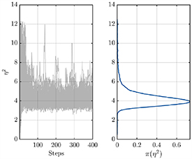
Figure 3. Bayesian inference via UQLab [36] with uniform prior  : MCMC paths and posterior distribution of η2 (mean: 4.1235, std: 0.5864, median: 4.0357, 5th percentile: 3.3645, 95th percentile: 5.1811).
Download figure:
Standard image High-resolution image3. Probabilistic tipping diagrams
The prior physical ranges from section 2.1 and the probability distribution obtained by the Bayesian inference method in section 2.2 can now be used to generate probabilistic tipping diagrams. These are intended to visually support the assessment of how far the system is from tipping.
3.1. Tipping diagrams based on prior parameter ranges
We first show a probabilistic representation of the equilibrium curve when using the prior parameter range (6) for η2. In figure 4(a), we plot the steady states (5) for  , i.e. η2 is assumed to be uniformly distributed on the interval
 ![$[0.6,12.3]$](https://content.cld.iop.org/journals/1748-9326/17/7/075002/revision1/erlac7602ieqn38.gif) . The grey scale shows the mass levels indicating the percentages of realisations that are covered by the corresponding area. These are calculated numerically based on
. The grey scale shows the mass levels indicating the percentages of realisations that are covered by the corresponding area. These are calculated numerically based on  realisations. The red solid line here and in subsequent figures indicates the bifurcation curve for the cusp value
  . The black solid line corresponds to the mean
  and obeys the characteristic S-shape described in section 2. Note that, due to the nonlinearity, the range of values of µ is squeezed and expanded depending on the salinity difference x.

Figure 4. Probabilistic bifurcation diagrams for Stommel–Cessi model according to prior and posterior parameter distribution from Bayesian inference on synthetic data from section 2.2.1. The uncertainty in the key model parameter η2 has been drastically reduced resulting in a substantial narrowing of the range of tipping behaviour. For this and subsequent diagrams: the grey scale shows the mass levels indicating the percentages of realisations that are covered by the corresponding area. The red line corresponds to the cusp  case (no tipping for
  , two TPs for
  ).
).
Download figure:
Standard image High-resolution imageIn this case a wide range of behaviours is possible. A significant number of realisations show tipping at a relatively low value of the freshwater flux (say µ < 1), while a few realisations have  and so have no tipping behaviour, but nevertheless show a large AMOC decline in response to small increases in water flux. Such a decline would be expected to have significant climate impacts but would be more reversible than if a TP had been crossed.
The parameter distribution assumption over the prior physical range (6) can have a major impact on the prior probabilistic tipping diagram that emerges. This is shown in the appendix which recalculates the probabilistic bifurcation diagram 4(a) with the uniform prior distribution replaced by a truncated normal distribution. Therefore, confident conclusions about the likelihood of AMOC tipping cannot be made based purely on knowledge of the physical range (6). The Bayesian step delivers a more robust distribution for η2.
3.2. Tipping diagrams based on Bayesian parameter inference
Figure 4(b) shows how the probabilistic tipping curve is constrained by the Bayesian inference step. It shows the sample-based probabilistic tipping diagram according to the posterior distribution of η2. Here, we use a sample of size M = 20100 drawn from the posterior distribution exported from our UQLab result. The area in which the bifurcation curves lie is far narrower than under the uniform distribution assumption (figure 4(a)). In particular the range of fresh water flux µ for which a strong AMOC can be maintained is much narrower, and large AMOC changes at extremely low values of µ have been ruled out. Note that the regime without TPs is no longer present within  of the realisations. The Bayesian step has drastically reduced the dependence of the TP estimate on the somewhat arbitrary choice of prior distribution.
3.2.1. Visualisation of probabilistic TPs
Not only does the parameter uncertainty in η2 turn the bifurcation curves into random objects, but also the locations of the TPs themselves become uncertain. Histograms based on the posterior sample of η2 for critical values of the nondimensional freshwater flux (µ− and  ) and salinity difference (
 and
and  ) are depicted in figures 5(a) and (b) respectively.
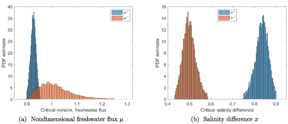
Figure 5. Histogram of critical values of the nondimensional freshwater flux and the salinity difference for the strong AMOC TP  and the weak AMOC TP
  based on a posterior sample of η2.
Download figure:
Standard image High-resolution imageBy putting together the critical values (µ−,  ) and (
 ,
,  ), we obtain an approximation of the 2D joint probability distribution of the strong
  and weak
  AMOC TPs (figure 6). The grey scale again indicates the ranges, in which the TPs lie for the indicated masses of realisations of η2. Figure 6 reveals that the location of the TPs varies significantly, even for the sample values from the posterior distribution of η2, as was suggested by figure 4(b).

Figure 6. Probabilistic location of strong and weak AMOC tipping points (TPs)  and
and  based on posterior sample of η2.
Download figure:
Standard image High-resolution image3.2.2. Probabilistic visualisation of cusp bifurcation
By passing from a 2D representation as in figure 4(b) to a 3D representation and again using the grey scale colour code as before, we provide a probabilistic visualisation of the fold curves with corresponding values of η2 (see figure 7). Observe again the occurrence of a cusp bifurcation at  (red line): In front of this curve (
 ), there is no value of the nondimensional freshwater flux for which bistability of the system occurs, i.e. no TPs exist. The classical S-shape double fold curve can be observed behind the red curve (
 ).
).

Figure 7. Probabilistic fold curves in 3D (only 
 posterior samples used).
Download figure:
Standard image High-resolution imageAn alternative view on the probabilistic cusp bifurcation behaviour is provided in the appendix. It shows that the range of the fresh water flux µ for which a strong AMOC can be maintained is much narrower for the posterior sample. For further visual insights combining the probabilistic bifurcation diagram with the probabilistic location of the TPs, see figure 11 in the appendix.

Figure 8. Prior and posterior predictive distribution (first half of time depicted). Green synthetic data points are more narrowly comprised by posterior predictive (dark blue) indicating qualitative improvement within inference process on η2.
Download figure:
Standard image High-resolution image
Figure 9. Qualitatively different shape of probabilistic fold curves for  (truncated normal distribution over physical range (6)) compared to the shape in figure 4(a) for a uniform parameter distribution. The red line corresponds to the
  case (no tipping for
  , two TPs for
  ).
).
Download figure:
Standard image High-resolution image
Figure 10. Visualisation of critical flux values µ− and  , corresponding to the posterior sample of η2 (upper and lower grey scale curves, respectively). The dotted lines show the range of bifurcation positions using a uniform prior distribution for η2. The red line indicates the cusp case
  .
.
Download figure:
Standard image High-resolution image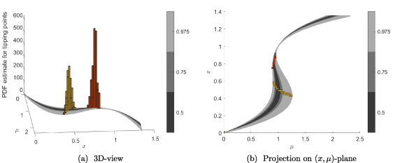
Figure 11. Probabilistic bifurcation diagram for Stommel–Cessi model resulting from Bayesian inference on synthetic data from section 2.2.1 with probabilistic TPs locations (red:  , yellow: µ−).
Download figure:
Standard image High-resolution image
4. Discussion and outlook
We have proposed new techniques to understand how uncertainty in model parameters translates to uncertainty in the location of climate TPs. We have illustrated our methods using a simple AMOC box model, focusing on a particular parameter η2 that is difficult to estimate directly from observations. We have described a Bayesian approach to obtain a probabilistic estimate of the model parameter(s) and shown that, given a suitable observed timeseries, this can drastically narrow uncertainty in the location of the bifurcation point. We have proposed visualisation techniques to understand the impact of parameter uncertainty on bifurcations. The key advances shown by our work are:
- First, that the Bayesian method produces a distribution for the unknown model parameter η2 that dramatically narrows the range of η2 compared to several reasonable choices of prior, and that the posterior is rather insensitive to the choice of prior.
- Secondly, that the resulting posterior distribution of η2 also results in significantly narrowed uncertainty in the nature and location of the AMOC TPs.
- Thirdly, that timeseries data can provide strong constraints on the TPs, even if they are sampled from a period when the AMOC was well away from a TP.
- Finally, we have presented a number of visualisations to aid interpretation of the probabilistic TP behaviour.
Our approach is rather generic. It might also prove valuable in the assessment of other tipping elements of the Earth System, or indeed in other scientific disciplines such as neuroscience and epidemiology, where parametric uncertainty is common.
Our results show promise that suitable proxy timeseries may be used to give valuable constraints on AMOC TPs, even if the timeseries only cover the Holocene period when the AMOC has been relatively stable. Our goal here has been to illustrate the promise of the approach using a simple modelling framework. Several caveats exist that require further work before the method can be used to develop a robust probabilistic assessment of AMOC TPs. In particular:
- A long enough observed timeseries would be required to adequately constrain the model parameter(s). We have used a synthetic timeseries of length around 1400 years. We note that proxy AMOC timeseries of the required length are available [44], but application of these goes beyond the scope of this paper.
- It is important that the underlying model adequately captures the dynamics of AMOC tipping. While the 2-box model may be too simple as it does not allow a salinity-driven AMOC through the net evaporative nature of the Atlantic basin [45], it has recently been shown that a slightly more complex box model has quantitative skill in reproducing the dynamics of AMOC tipping in a GCM [6]. The selection of an appropriate simple model as an emulator or surrogate model for GCMs is likely to be an important step in assessing likelihood of tipping in the real world [18, 29, 31].
- We have illustrated our method using a single uncertain parameter, with other parameters assumed to be known. The Bayesian approach can be readily generalised to more parameters, as shown for a simple climate-carbon-AMOC model by [22]. For the AMOC, credible underlying models exist, whose parameters can mostly be well constrained by observations [6], helping to keep the number of uncertain parameters to a level where computational cost is not a decisive factor. Similar approaches for higher dimensional systems may rely on carefully chosen and optimised numerical methods.
- As the dimension of the parameter space increases, visualisation becomes more difficult. However, the diagrams shown here are valuable as 'cross-sections' of the parameter space, to build understanding of which parameter regimes entail high likelihood of tipping. In the case of a second uncertain parameter, a three-dimensional extension of figure 6 would provide a useful summary of the TPs as a function of physical climate variables, within which we obtain a two-dimensional manifold instead of a one-dimensional curve, so that a suitable two-dimensional projection would provide a 'heat map' of the location of the TPs.
For future research, it will be valuable to explore whether useful constraints can be derived from available Holocene AMOC timeseries (e.g. [44]), or from deeper-time proxies where AMOC tipping may have occurred. Application of current methods to other climate TPs [46, 47] may also be productive.
The importance of high impact, low likelihood climate outcomes, including TPs, is only just emerging as a key element in climate risk assessments [48], and improved methods will be required to assess whether such outcomes could plausibly occur in future climates. The techniques developed here show promise in that we can use knowledge of past behaviour to better understand likelihoods of such events in future.
Acknowledgments
The authors acknowledge support of the EU within the TiPES project funded by the European Union's Horizon 2020 research and innovation programme under Grant Agreement No. 820970. This is TiPES publication #131. RW was also supported by the Met Office Hadley Centre Climate Programme, funded by BEIS.
Data availability statement
The data that support the findings of this study are openly available at the following URL: https://github.com/kerstinLux/parametricUncertaintyAMOCtipping.
Appendix
Information on Bayesian setup
If we denote the numerical solution of the ODE model (3) (with  and µ = 0.85) at time
  ,
,  , by
, by  , the synthetic 'truth' time series
  , where
  , i.e.
  , can be written as:
where  ,
,  , with an unknown variance σ2, represent the discrepancy between observations and model forecasts. For simplicity, we assume an additive Gaussian discrepancy also for
  . We obtain the log likelihood function
  as in [36, p 6], which reads as:
where  is the number of data points in the synthetic 'truth' time series and
  denotes the vector of the numerical solutions of the ODE (3) at times tj
,
denotes the vector of the numerical solutions of the ODE (3) at times tj
,  , with parameter η2.
Comparison of prior and posterior predictive distribution
We take the Bayesian inference settingfrom section 2.4 and compare the prior and the posterior predictive distributions in figure 8. The posterior predictive distribution gives a narrower prediction of the green synthetic data points than the prior distribution, indicating a qualitative improvement of the parameter estimate over the inference process.
Major impact of prior parameter distribution on prior tipping behaviour
The assumed distribution within the prior parameter range (6) could have a major impact on the (prior) probabilistic tipping curve. If we assume a truncated normal distribution over the physical range (6) for η2 with mean 6.45 and standard deviation of 1, i. e.  instead of the uniform parameter distribution in figure 4(a), we obtain a narrower area for the bifurcation curves being comprised by the bistable regime
  (figure 9). Whereas a value of
  is within the range where
  of the realisations lie for the uniform distribution (figure 4(a)),
  is not contained in
  of the realisations with the truncated normal distribution
  . With this choice of parameter distribution nearly all cases are bistable, and very few tip to the weak AMOC branch for µ < 1.
This problem of major differences in the shape of the bifurcation curve is removed after applying our Bayesian inference procedure from section 2.4. If more information on the parameter distribution is known in advance, of course, a more tightly constrained prior further reduces the standard deviation of the posterior parameter distribution and is thus preferable. For more details on prior assessments, see [49].
Alternative visualisation of probabilistic cusp bifurcation behaviour
The probabilistic cusp bifurcation behaviour can be visualised by plotting realisations of the posterior distribution of the uncertain model parameter η2 against the corresponding critical nondimensional freshwater flux values (figure 10). Again, the grey scale indicates the spread of the realisations of η2 and the red line the cusp value of  . The black dotted line shows the critical nondimensional freshwater flux values according to the prior distribution of η2. Note again that the range of the fresh water flux µ for which a strong AMOC can be maintained is much narrower for the posterior sample.
Holistic probabilistic tipping visualisation
In a holistic visualisation (figure 11), we combine insights gained from previous diagrams. We combine the probabilistic bifurcation diagram inferred by our Bayesian inference (figure 4(b)) with the probabilistic location of the TPs shown in figure 6. A top-down view is shown in figure 11(a). The grey scale is used for the probabilistic bifurcation curves as before and the probabilistic location of the TPs is depicted using a histogram based on the posterior sample of η2 in the third dimension (figure 11(b)).
Footnotes
- 5
- 6
https://de.mathworks.com/help/matlab/ref/ode45.html, last checked: 12 August 2021.