

Abstract
The impact of climate variability on the water requirements of crops is a key issue in a globalized world with unprecedented population and unevenly distributed water resources. Changes of hydro-climatic forcings may have significant impacts on water resources use, considering the possible effects on irrigation requirements and crop water stress. In this work, a comprehensive estimation of crop water requirements over the 1970–2019 period is presented, considering 26 main agricultural products over a 5 arcmin resolution global grid. The assessment is based on a daily-scale hydrological model considering rainfed and irrigated scenarios, driven by hydro-climatic forcings derived from ERA5, the most recent climate reanalysis product within the Climate Change Service of the Copernicus Programme. Results show the heterogeneous impact of climate variability on harvested areas of the world, quantified by water stressed days and irrigation requirement rates. Increases of irrigation requirement rates were found on more than 60% of irrigated lands, especially in regions like South Europe, North-East China, West US, Brazil and Australia, where the mean rate increased more than 100 mm yr−1 from 1970s to 2010s. The daily analysis of water requirements shows that crops require significantly more days of irrigation per season, especially in Europe, Africa and South-East Asia. Statistically significant trends of water stress duration were found over 38% of rainfed croplands, while only 6% of croplands has been affected by negative trends and shorter stress duration, mainly in India, Malaysia, North Europe and coastal regions of central western Africa.
Export citation and abstract BibTeX RIS

Original content from this work may be used under the terms of the Creative Commons Attribution 4.0 license. Any further distribution of this work must maintain attribution to the author(s) and the title of the work, journal citation and DOI.
1. Introduction
Agriculture is one of the leading human activities and one of the most exposed to climate change. The growth of crops is highly related to climate conditions, whose variability can lead to water stress and production losses [1]. In fact, the spatio-temporal variability of precipitation and evapotranspiration has significant consequences on crop water requirements and on irrigation [2]. The assessment of crop water needs at large spatial scales is essential to adopt proper water-related policies [3], to promote an optimal use of water resources and to address land and agricultural management.
Remote sensing offers new possibilities to apply hydrological models at large spatial scales, with a relatively high resolution. The uniform quality of satellite data fits the need of global models, enabling the quantitative assessments of key variables of the water cycle at the global scale [4]. The ERA5 reanalysis dataset from the Copernicus Climate Change Service, based on assimilation of remote sensing and ground measurements, provides several hydro-climatic variables with a high spatio-temporal resolution, that can be useful in coupled hydrological-agricultural applications [5].
The temporal variability of crop water requirement is a key topic in the study of climate effects and adaptation strategies. The Agricultural Model Intercomparison and Improvement Project (AgMIP) [6], for example, tested different available models in the production of future climate scenarios for agriculture at the global scale with 0.5° grid resolution. Other few works analyzed the climate-driven changes of crop evapotranspiration in the recent past. Ruane et al [7] examined the performance of different climate datasets in agricultural large-scale models within the AgMIP project, considering four crop types and different combinations of climate forcings/crop gridded datasets. Recently, Chiarelli et al [8] estimated the global water requirements for years 2000 and 2016, providing monthly crop-specific results. Other studies focused on national or subnational scales, e.g. the assessment by Yin et al [9] applied to China from 1982 to 2015. Yet, there is still a lack of works that use the most up-to date remote sensing dataset to improve the accuracy of multiannual global evapotranspiration assessments at the daily time scale.
The present work aims at filling this gap, assessing the impact of climate variability on crop water requirements and on the duration and intensity of water stress, across the period 1970–2019. The research questions that this letter wants to address are: has climate change already impacted rainfed and irrigated agriculture? Is there statistical evidence of an increase in the duration and intensity of water stress? Where have irrigation requirements per crop changed more markedly?
To address these questions, an existing coupled soil water balance and crop growth model [10] has been used to estimate the daily actual evapotranspiration of 26 main crops for five decades, using ERA5 climate data. The daily scale enables the quantification of the effects of hydro-climatic fluctuations on the timing and duration of water-stressed periods. In this work the information on rainfed and irrigated cropland areas is fixed in time, allowing to focus on the temporal variability of hydro-climatic drivers alone. Consequently, the variables analyzed are, as much as possible, not dependent on the extent of the harvested areas per pixel, e.g. water depths are considered rather than volumes. The estimation of the temporal evolution of water volumes, which requires the knowledge of harvested and irrigated areas per crop in time, is beyond the scopes of this work.
2. Methods
The present work aims at analyzing the evolution of crop actual evapotranspiration, ETa, at the global scale as dependent on the temporal variations of climate forcings. The ETa is estimated separately over rainfed and irrigated areas, considering in the latter case the supply of the minimum amount of irrigation to avoid water stress in crops. To this purpose, a coupled vegetation and soil water balance model based on the Food and Agriculture Organization (FAO) guidelines [11] was used. The model, stemmed from Tuninetti et al [12] and presented in Rolle et al [10], is here applied globally from 1970 to 2019.
The assessment is based on the gridded harvested areas of 26 main crops and related monthly growing seasons from MIRCA2000 [13], available at the spatial resolution of 0.0833° (about 9 km at the Equator). The geographical distribution and the extension of croplands, as well as the irrigation equipment, are fixed in time. The 26 crops are listed in Rolle et al [10] and include perennial crops resulting from permanent cultivations (e.g. fruit trees) and temporary crops which are sown and harvested during the same year, even more than once (e.g. maize and wheat) [14]. Temporary crops are assumed to be sown and harvested on the mean days of the month, in agreement with Tuninetti et al [12]. The growing season of perennial crops reflects the annual vegetative cycle of the plants. Even if a comprehensive assessment could be affected by crop change, migrations or switches, the lack of information at the global scale prevents consideration of these factors in the present analysis.
2.1. Daily climate data
The model runs at a daily time step using precipitation (P) and reference evapotranspiration (ET0), defined as the evapotranspiration from an ideal well-watered grass surface [11], to compute the soil water balance and to assess the crop actual evapotranspiration. The simulation covers the period 1970–2019 and is based on the climate data from ERA5, i.e. the global reanalysis dataset produced by the European Centre for Medium-Range Weather Forecast within the Copernicus Climate Change Service [15, 16]. The reanalysis uses the information from ground measurements and the global satellite network, exploiting the growing availability of remote sensors over the last two decades [17].
Although ERA5 includes results since 1950, the present analysis starts in 1970 in order to avoid uncertainties related to previous periods [18]. The climate data were downloaded at the original resolution of 0.25° (about 30 km at the Equator) and processed with the Climate Data Operators (CDO) [19] to match the MIRCA2000 grid. The CDO tool offers specific methods of interpolation to redefine the resolution of each climate variable.
Daily precipitation was calculated by summing hourly rainfall from 1:00 am to 0:00 am in each day. Daily reference evapotranspiration,  (in mm d−1), was calculated according to the Hargreaves–Samani method [20], i.e.
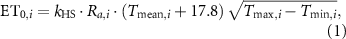
where  is an empirical coefficient (fixed to 0.0023 in the original formula [20]),
  ,
,  and
and  are respectively the maximum, minimum and mean temperatures for the ith day (in °C) and
  is the equivalent evaporation (in mm), calculated as ratio between the top-of-atmosphere radiation and the latent heat of vaporization of water (1/λ = 0.408). Temperature and radiation are daily-averaged ERA5 data. The value 17.8 in equation (1) imposes a null
  when
when  .
.
Although Hargreaves–Samani is one of the methods suggested by FAO to calculate ET0 [11], the empirical coefficient kHS in equation (1) was calibrated for each pixel, in order to reproduce annual values of  available from a reference application of the Penman–Monteith method. According to the procedure described by Rolle et al [10] for the calibration on year 2000, the CRU Time-Series global data [21] was used to calculate the annual deviations between Hargreaves–Samani and Penman–Monteith, as ratio between ET0,PM and ET0,HS (mm yr−1) in each pixel. The final grid of kHS was obtained as multiplying the original value (0.0023) by the 1970–2019 mean deviations. The calibration was performed considering all the 70 years, in order to include the decades of maximum density of ground sensors used by CRU (1961–1990) [22], and the recent years with most active satellite sensors on which ERA5 in based [17]. This simplified method for the assessment of ET0 limits the uncertainty related to using many input variables, while remaining consistent with ground-based annual data of Penman–Monteith ET0.
2.2. Soil properties
The amount of water a crop can draw for its needs is related to the soil properties of water-holding capacity [11]. The field capacity (θfc) [ /
/ ] is the upper limit of soil moisture after drainage, while the wilting point (θw
) [
] is the upper limit of soil moisture after drainage, while the wilting point (θw
) [ /
/ ] represent the dry condition at which the crop stops evapotranspiration. The difference between the two limits is called available water capacity (AWC) and represents the maximum quantity of water that crops can withdraw from the soil.
The global SoilGrids dataset (250 × 250m resolution) [23] was used to set the global AWC over croplands. The original grid was upscaled to obtain a 0.0833° grid, matching the MIRCA2000 resolution. Pixel values were computed averaging the SoilGrids pixels containing croplands according to the global soil classification from the Copernicus Land Service [24]. Since SoilGrids provides data for different soil depths, the final AWC was further calculated as a mean between the upscaled grids up to 1 m depth, to set a representative value of available water capacity per unit of soil volume in the rooting zone.
Each crop has a specific tolerance threshold to water stress: the soil moisture threshold of incipient water stress (θ*
) [ /
/ ] depends on the crop-specific sensitivity to soil water deficit, i.e. the difference between the field capacity upper limit and the actual water content in the soil, as described by Allen et al [11]. The crops that are more sensitive to soil water deficit reach water stress in wetter soils, while the same deficit still represents a sufficiently wet condition for the less sensitive crops.
2.3. Evapotranspiration and irrigation
According to Allen et al [11], crop development occurs in four phases, which are associated to specific evapotranspirative non-dimensional coefficients (kc ) governing the well-watered evapotranspiration rate. The crop-specific details of the growing phases are provided by Chapagain and Hoekstra [25] for ten climatic regions of the world, according to the agro-ecological classification proposed by FAO [26]. The daily crop evapotranspiration (ETc) (mm d−1) is defined for well-watered fields as the product between reference evapotranspiration (ET0) and the crop-specific coefficient kc . The daily actual evapotranspiration (ETa) (mm d−1) also takes into account the reduction due to water stress when soil moisture drops below θ* .
According to the methodology proposed by FAO [11], ETa is calculated according to

where ET0 is the reference evapotranspiration of the i day (mm d−1), kc is the non-dimensional crop coefficient that depends on the development phase, and ks (–) is a water-stress coefficients depending on the daily soil moisture condition and to the crop-specific sensitivity to soil moisture decreases [10]. When ks = 1 no water stress occurs, while ks = 0 means that the crop has reached the wilting point.
The irrigation requirement (I) is consistent with the definition given in Rolle et al [10], i.e. it is the minimum water depth needed by the crop to avoid water stress and keep evapotranspiration at ETc . Crops harvested on areas equipped for irrigation (AEI) are supposed to receive a daily quantity of water to avoid water stress, i.e. to reach the minimum soil moisture at which water stress does not occur.
2.4. Initial soil moisture
For temporary crops, the initial soil moisture at the sowing date (θsow) needs to be defined. Considering the lack of information about the cropland use before the sowing date, the corresponding moisture cannot be obtained from the soil water balance. Previous studies used different solutions to address this problem: Chiarelli et al [8] used an initial soil moisture equal to 50% of AWC; Siebert et al [27] proposed a simplified water balance on fallow lands with kc = 0.5; Rolle et al [10] assumed that each growing season starts with soil moisture at field capacity.
In this study, a sensitivity analysis was performed to quantify the impact of initial soil moisture on the final estimations of ETa and I for temporary crops. Two simulations were performed assuming the two limit values of initial soil moisture, θsow= θfc and θsow= θwp in the starting day of each temporary growing season. The global area-weighted average of ETa and I rates (mm yr−1) were calculated for the 1996–2005 period, on rainfed and irrigated areas respectively. Results show that the global actual evapotranspiration of temporary crops is 12% lower when the growing seasons start at wilting point, compared to the 'field capacity' hypothesis. Moreover, irrigation requirement (excluding rice) is about 3% higher when all temporary seasons start at wilting point.
To reduce the value of the uncertainty related to soil moisture at the sowing date, soil moisture data were used in this work, to be consistent with the actual weather conditions, again provided by ERA5 [28, 29] for different soil layers. Assuming 0.2 m as the standard effective rooting depth for the water balance calculation at the sowing date [30], the monthly soil moisture grids were calculated as the average between the first two layers (0–7 cm and 7–28 cm respectively). For each sowing day, the soil moisture was calculated as the fraction of the 'soil saturation upper limit' dataset from SoilGrids, equal to the ratio between the monthly soil moisture and the saturated moisture from ERA5. Since ERA5 does not provide any information about maximum soil water capacity, the saturated limit was set using the maximum values for the 1970–2019 period in each pixel. When the initial soil moisture turned out to be higher than field capacity, the θfc value was used.
2.5. Water requirement daily statistics
The use of daily hydro-climatic data over a 70 years period enabled long-term simulations at the daily time scale, which in turn allowed to perform analysis of daily results. For each crop, the number of precipitation events (PD, i.e. precipitation days) with rainfall greater than 2 mm d−1 was computed for the growing season of every year from ERA5 data. PD was compared to the number of days in which the crop requires irrigation (ID, i.e. irrigation days), considering a minimum modeled requirement of 2 mm d−1. For perennial crops, PD and ID were computed throughout the whole year, while for temporary crops they referred to the growing periods.
The PD and ID values were also aggregated at different spatial scales: to this aim, the aggregated results were averaged over the area of interest, using the extension of area equipped for irrigation as weight.
In rainfed areas, where no irrigation occurs to avoid the daily water stress, the number of water stressed days (days in which ks < 1) for each crop was computed and indicated with SD. In order to compare pixels with different cropland extensions and compositions, a proper index was defined considering all crops grown in the pixel, i.e.
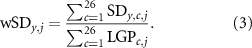
wSD (–) quantifies the annual number of water stress days of year y on the j pixel, calculated as the ratio between the sum of SD on rainfed areas for the 26 crops, and the sum of the corresponding lengths of growing periods (LGP in days) in the same pixel. The wSD index has been introduced to normalize the total number of water stress days per pixel. The rainfed scenario ensures that no other water inputs occur but rain, allowing to test the effect of dry periods on cultivations.
3. Results and discussion
3.1. Temporal variability of irrigation requirement
The irrigation requirement (I) is strongly related to the precipitation availability. More than on the total rainfall rate, I depends on how rainfall is distributed across the growing season: more irrigation is required during long dry periods, while frequent small rainfall events may keep soil moisture far from stress levels. The number of days requiring irrigation per growing season (ID) depends on the crop type, on the geographical position and on the harvesting calendars. This variable and the seasonal number of precipitation days (PD) referred to the maize growing seasons, were computed and aggregated in different areas of the world (figure 1). A t-Student test was performed to highlight significant temporal trends for ID, with a level of significance of 5%. Positive trends of ID were found to be statistically significant in Europe, East-Asia, South-East Asia, West Asia, South America, Sub-Saharan and North Africa. In the Southern and Eastern zones of Europe, trends of ID are marked because of the combination of ET0 increments and strong decreases of PD (in some cases, −35% from 1970s to 2010s), as confirmed by Seneviratne et al [31]. In Northern Africa, precipitation is very low (both considering annual rates and number of events): therefore, the ID increment through the years is mainly driven by the ET0 trend. Significant ID trends were found in Sub-Saharan Africa, West and East Asia and Oceania, with different slopes.

Figure 1. Temporal variability of annual precipitation days (circles) and days requiring irrigation (crosses) for the growing of maize (1970–2019). The slopes of the green and blue lines show the linear trends of rainfall days and irrigation days for maize, respectively. The analysis is performed in 15 areas of the world, defined by the UN classification. In the legend, GS stands for growing season.
Download figure:
Standard image High-resolution imageThe slightly negative ID slope in North America results from the combination of two opposite scenarios: in the East part of Canada and USA a precipitation increment caused a considerable reduction of irrigation requirement, while on the Western regions the opposite occurs (not strong enough to be detected on a sub-continental scale).
Changes of PD from ERA5 are reflected in other studies about trends of wet days, like the global analysis by Rajah et al [32]. Global projections from the last IPCC report [33] shows high confidence that future changes of wet days will confirm the trends of the last decades.
An increase in time of the number of days requiring irrigation (ID) leads to two main consequences. First, higher ID often implies increment of irrigation requirement volumes over the growing season, because the final estimation results from a larger number of stress events. Second, the crop requirement in many areas of the world may not be entirely satisfied with the current irrigation calendars, especially for those crops requiring frequent irrigation (e.g. vegetables or pulses).
The temporal variation of irrigation requirement rates (I) was analyzed for the 26 crops under study, calculating daily series from 1970 to 2019. The analysis reveals that I increased in 62% of areas equipped for irrigation, comparing the mean annual rates of 1970s and 2010s decades (figure 2).
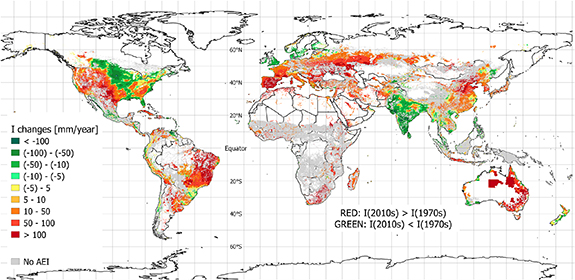
Figure 2. Changes of mean annual irrigation requirements (I) (mm yr−1), comparing 1970s and 2010s. The map colors describe how much (red) or less (green) irrigation is required over the AEI between the two decades, comparing the ten years AEI-weighted average requirement of 26 crops.
Download figure:
Standard image High-resolution imageThe increment is higher than 10 mm yr−1 on more than 53% of global irrigated areas. The highest increments of mean annual I (>100 mm yr−1 from 1970s to 2010s) were found in South Europe (especially in Spain, Italy, South France, Balkan peninsula and Ukraine), North-East China, the eastern part of Australia, Brazil, and the western part of USA.
In 29% of irrigated areas, the irrigation requirement decreased from 1970s to 2010s for more than −10 mm yr−1. Most of these areas are concentrated in South Asia and in the central part of USA, from North Dakota to Mississippi. In the first case, less irrigation is required because of the combined effect of mean ET0 decrease and precipitation increments (especially in the Indo Valley and Northern India), while the result in USA depends mostly on the greater precipitation availability (+100 mm yr−1 from 1970s to 2010s), that compensated the increment of ET0 (+10 mm yr−1).
A more detailed analysis of the I variations was performed considering some relevant crops.
In the supplementary material (figure 1S available online at stacks.iop.org/ERL/17/044017/mmedia), the temporal variability of mean daily irrigation requirements of citrus is shown, comparing the Aragon-Catalonia region (Spain), Israel and Cuba. The mean daily I has generally increased comparing 1970s and 2010s (e.g. +50% in Spain during summer, from about 2 mm d−1 to more than 3 mm d−1). The period of irrigation has also increased through the years in the three countries. In the last decades, citrus required irrigation in the early-spring period (which was not necessary in the 1970s) and higher irrigation rates during the spring and autumn periods.
3.2. Changes of crop irrigation requirements over latitudes
The comparison of crop-specific rate of irrigation requirement between 1970s and 2010s shows a heterogeneous pattern. The variability of climate forcings has different impacts on I depending on the latitude, because of the heterogeneous changes of P and ET0. The crop-specific comparison shows that in most of the northern AEI, above 30° N, more irrigation is required in 2010s than in 1970s. As shown in figure 3, going from North to South, all the croplands require more irrigation except the fodder grasses (which are mainly harvested in the Eastern part of Canada and USA, where the I rate have decreased).

Figure 3. Variations of crop-specific irrigation requirements (mm) by latitude, between 2010s and 1970s. The box below shows the geographic distribution of crop areas equipped for irrigation (AEI): more than 90% of AEI are in the Northern hemisphere, most of which located between 20° N and 40° N.
Download figure:
Standard image High-resolution imageThe crop-specific analysis in the northern hemisphere shows higher increments of I from 1970s to 2010s for multi-seasonal temporary crops (e.g. wheat, which is harvested both in winter and spring-summer), especially in North-West America, Europe and North-Central Asia. Soybean requires quite the same amount of irrigation if comparing the two decades at these latitudes, as a result of the opposite effects of higher I in Eastern China and lower I in Eastern USA. Most of the irrigated areas from 30° N to Equator are in South-East Asia, except for some regions in Central America.
Most of the AEI in India and Pakistan requires less irrigation in 2010s than in 1970s: the irrigated croplands in these nations are favored by the changes of climate forcings, which lead to an advantageous scenario from the point of view of agricultural water needs. Considering the global scale, a hypothetical crop switch from North to South in Asia could be a beneficial solution, with a significant reduction of I. For example, we found larger increments of irrigation requirements in the Northern part of China, where most of the irrigated areas are concentrated and water is partly transferred from southern regions, through the South–North Water Transfer Project [34].
Less than 10% of irrigated lands are in the Southern hemisphere. The analysis of water requirement variability indicates very high increments of irrigation requirement for all the crops harvested in these regions. The combined effects of climate forcings on Oceania, Southern Africa and Southern America, lead to significant disadvantages in the irrigation practices in this hemisphere. The Amazon region appears to be quite unsuitable for irrigated agriculture from a climatic point of view [35] and results show high increments in the irrigation required by crops in this area. Contrary to the Northern hemisphere, irrigation requirement has increased more on the coolest regions going from North to South, mainly because of the strong reduction of mean annual precipitation (up to −300 mm yr−1 in Brazil, due to the combined effect of climate variability and deforestation [36]). The irrigation requirement of soybean appears to be less sensitive to climatic variability, as previously found in the Northern hemisphere.
3.3. Water stress trends on rainfed croplands
A trend analysis of crop water stress, induced by climate change, was performed on rainfed croplands. On these areas, precipitation is the only water input, and it is possible to quantify and compare the length and the severity of water-stress periods. Considering this, it is possible to relate the water stress to potential yield losses of rainfed crops.
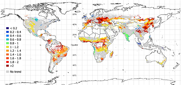
The annual water stress days (wSD) were calculated for each pixel containing rainfed crops, from 1970 to 2010, as described in section 2.4. A t-Student test was performed to highlight significant trends, with a level of significance of 5%. On a global scale, 38.1% of rainfed areas show statistically significant positive trends of annual water stress days, while significant decreases were found only for 6.7% of the rainfed areas.
As shown in figure 4, large part of East Europe and East China shows high trends of wSD, more than double in 2010s than in 1970s. In the Central Africa, high wSD increment depends on the fact that in 1970 rainfed areas were affected by very small stress: despite the water stress in 2010s still counts a few days per year, it should be noted that most of the croplands in Central Africa are rainfed, and these increments may lead to reduction of crop yield with significant consequences. South and East Europe are affected by significant increments of annual stress days. Some of these regions are densely harvested (e.g. Northern Italy, Spain and Ukraine), and high positive stress trends may limit the rainfed crop yield, affecting national crop productions. Western China shows a similar scenario, while in the central part of the nation the heterogeneous changes of precipitation availability led to a more complex scenario: increments of precipitation in Eastern Qinghai have diminished the water stress on rainfed areas.
Figure 4. Ratio between 2010s and 1970s mean annual stress days on rainfed areas. Warm colors indicate that the mean number of annual stressed days has increased during the last 50 years, while the cold colors describe the opposite scenario. Over grey areas, there is no significant trend of water stress days, according to the t-Student (level of significance of 5%).
Download figure:
Standard image High-resolution image
All the South America shows high positive trends of wSD, especially in the Amazon region. Despite the mean annual precipitation rate has slightly increased over the decades, the annual number of precipitation days has decreased (as shown in figure 1 for the maize season). Because of this situation, the low number of stressed days has more than doubled in many parts of Brazil and Colombia. India is one of the nations with the highest extension of rainfed areas. A large part of this region is affected by significant negative trends of annual ET0, resulting from the combined effect of factors: the falling of the difference between maximum and minimum temperatures, decrease of wind speed and increasing of cloudiness on the region [37]. The further general increase of annual precipitation rates, according to the ERA5 data, leads to significant decrease in the number of stressed days per year, particularly in the Southern part of the nation.
A similar analysis was performed to find significant trends of severe water stress, considering annual days close to wilting point (ks < 0.1). In this case, 16% of rainfed croplands show a significant positive trend (see supplementary material, figure 2S). In North America, most of the rainfed areas are affected by low trends of annual stress days, both positive (in the Western region) and negative (Minnesota, North Dakota and Missouri). However, the number of severe-stress days has increased in most of the Western rainfed croplands.
This means that, even if the annual duration of water stress did not significantly change (figure 4), water stress has become much more severe. High trends of severe stress were found in Spain, Ukraine, North-East China, South Africa and the Amazon region.
The analysis of water stress on rainfed croplands is particularly interesting for those countries with poor irrigation infrastructures. In these nations, water stress increments may have a huge impact on the local economy, with limited possibility of adaptation because of the technology gap. In contrast, important rainfed stress and consequent yield losses may induce developed countries to improve the irrigation efficiencies of their irrigation systems [38], equipping part of the rainfed fields for irrigation. As an alternative, nations may shift to alternative crops and varieties and/or shift planting dates in areas most affected by climate impacts, using crop migration as an adaptation strategy [39].
4. Conclusions
In this work, the impact of climate change on rainfed and irrigated agriculture has been examined through trend analyses of water requirements and water stress. Results show heterogeneous changes in the irrigation requirements of crops over the 1970–2019 period, both in terms of annual rates and in the number of days in which irrigation is required. On more than 53% of irrigated croplands, the irrigation requirement has increased more than 10 mm yr−1 comparing the 1970s and 2010s decades. Moreover, there is a statistically significant increase in the annual number of days requiring irrigation in most irrigated areas of Europe, East and West Asia, Africa and Oceania, mainly due to a decrease of precipitation events during the growing seasons.
The global analysis of temporal changes highlights also a decrease of annual irrigation requirements in some world areas, such as the intensively harvested areas in South Asia and North-East America, comparing the mean annual rates of 2010s and 1970s. Focusing on rainfed croplands, the temporal analysis highlights that 38.1% of areas are affected by statistically significant positive trends of annual water-stressed days, while significant negative trends were found on 6.7% of rainfed areas. On 6% of rainfed areas, the number of annual water-stressed days has more than doubled over the considered period (1970–2019) and 16% of rainfed areas show a statistically significant increment of severe water stressed days per year.
Most of the cereals harvested in North America and Europe required more irrigation in 2010s than in 1970s, especially rice and wheat. The increase of irrigation requirements is progressively higher moving from North to South for most of the crops, particularly for cereals. In India and Pakistan, however, the irrigation requirements generally decreased through the decades, especially for rice, wheat and sugar cane. Most of the irrigation requirements in the Southern hemisphere has highly increased, disadvantaging the irrigated agriculture respect to the Northern regions. In most of Europe, South-East Asia, Oceania and Sub-Saharan Africa, the number of days per growing season requiring irrigation has significantly increased, especially because of decreases in seasonal frequency of rainfall days.
The global analysis of changes in the agricultural water requirements confirms that hydroclimatic forcings have already affected crop evapotranspiration in the past decades, causing yield losses. As regards the fixed in time distribution of croplands, a more detailed analysis of water volumes will be enabled when new crop-specific data quantifying the temporal evolution of rainfed and irrigated areas will be available. However, the results here obtained are already relevant to understand the climate-driven trends in water requirement. Results presented here are useful in the choice of adaptation strategies to climate change in agriculture at large spatial scales and may support the decisional process leading to policies of water and agriculture management and food production. These actions are, in fact, particularly complex in an increasingly globalized world, where nations are dependent on each other for food production and tightly interconnected by international trade.
Data availability statement
The data that support the findings of this study are openly available.