

Abstract
Fine particulate matter (PM2.5) is widely concerned for its harmful impacts on global environment and human health, making air pollution monitoring so crucial and indispensable. As the world's first open, real-time, and historical air quality platform, OpenAQ collects and provides government measurement and research-level data from various channels. However, despite OpenAQ's innovation in providing us with ground-measured PM2.5 worldwide, we find significant data gaps in time series for most of the sites. The incompleteness of the data directly affects the public perception of PM2.5 concentration levels and hinders the progress of research related to air pollution. To address these issues, a two-step hybrid model named ST-SILM, i.e. spatio-temporal model with single exponential smoothing-inverse distance weighted (SES-IDW) and long short-term memory (LSTM), is proposed to repair the missing data from PM2.5 sites worldwide collected from OpenAQ from 2017 to 2019. Both spatio-temporal correlation and neighborhood fields are considered and established in the model. To be specific, SES-IDW were firstly used to repair missing values, and secondly, the LSTM network was employed to reconstruct the time series of continuous missing data. After the global ground-measured PM2.5 was reconstructed, the light gradient boosting machine model was applied to remote sensing estimation of the original ground-measured PM2.5 and of the reconstructed ground-measured PM2.5 to further verify the performance of ST-SILM. Experiment results show that the estimation accuracy of the reconstructed dataset is better (R2 from 2017 to 2019 increased by 0.02, 0.02, and 0.01 compared with the original dataset). Therefore, it is concluded that the proposed model can effectively reconstruct data from PM2.5 sites worldwide.
Export citation and abstract BibTeX RIS

Original content from this work may be used under the terms of the Creative Commons Attribution 4.0 license. Any further distribution of this work must maintain attribution to the author(s) and the title of the work, journal citation and DOI.
1. Introduction
The Earth has been suffering from atmospheric pollution for a long time. Outdoor air pollution was in the list of first-class carcinogens in the World Health Organization's International Agency for Research on Cancer List of carcinogens for reference published on 27 October 2017 (https://monographs.iarc.who.int/list-of-classifications). Among all the outdoor air pollution, PM2.5 (i.e. particulate matter with aerodynamic equivalent diameter less than 2.5 µms) has caused particularly serious damage to human health, with a high mortality (Kim 2004, Neidell 2004, Kampa and Castanas 2008, Eze et al 2014, Guo et al 2017, Mannucci and Franchini 2017, Hamanaka and Mutlu 2018, Hime et al 2018, Nhung et al 2018, Glencross et al 2020). Studies have confirmed that PM2.5 also has an impact on human psychology (Dolan and Laffan 2016, Pun et al 2017, Wang et al 2017, Liu et al 2018, Liu and Salvo 2018), economy (Chang et al 2016, Li and Peng 2016, Aragón et al 2017, He et al 2019) and society (Fehr et al 2017, Younan et al 2018, Shi and Guo 2019, Burkhardt et al 2020). Monitoring PM2.5 concentrations is therefore crucial and indispensable.
At present, an important way to monitor PM2.5 is site monitoring, but monitoring sites mostly concentrate in a local area, such as a city or a country. Innovatively, the OpenAQ (https://openaq.org/#/about) platform collects and provides government measurement and research-level data from various channels (Hasenkopf et al 2015). Some studies have been carried out based on OpenAQ. Manning et al used aggregate data from OpenAQ to study daily patterns of global PM2.5 (Manning et al 2018). Berman and Ebisu obtained air pollution measurements from OpenAQ and studied the changes in air pollution in the United States during COVID-19 (Berman and Ebisu 2020). Despite OpenAQ's innovation in providing us with ground-measured PM2.5 worldwide, we find significant data gaps in time series for most of the sites, as it is usually unrealistic to obtain continuous, uninterrupted, and fully consistent data due to communications, equipment, and electrical failures or cyberattacks (Yu et al 2020). Therefore, we lack an effective global monitoring site dataset. The incompleteness of the data directly affects the public perception of PM2.5 concentration levels and hinders the progress of research related to air pollution. To mitigate the damage caused by air pollution and to better serve research related to air pollution, we need a more complete and accurate global ground-measured PM2.5 dataset to overcome the challenges posed by data gaps.
Several interpolation and machine learning models have been used to repair the missingness in spatio-temporal data, which can be broadly divided into spatial, temporal, and spatio-temporal repair. Spatial repair refers to the reconstruction of missing data through the spatial correlation between the known data, where the most widely used method is Kriging. As early as 1994, Rossi et al applied Kriging to remote sensing geostatistical interpolation (Rossi et al 1994). Moreover, inverse distance weighting (IDW) is also a widely used method. In 2016, Shareef et al applied this technology to optimize air quality monitoring networks (Shareef et al 2016). Temporal repair refers to the reconstruction of missing data through the distribution of historical data at a given location. The autoregressive integrated moving average (ARIMA) model (Velicer and Colby 2005) and simple exponential smoothing (SES) model (Gardner 2006) are both commonly used in it. However, it is difficult to obtain a satisfactory reconstruction result if only the spatial dimension or the temporal dimension is considered. Therefore, some studies have extended repair approaches to those which can consider both dimensions. For example, Chen et al rebuilt the continuous cloud-free Landsat images by spatio-temporal weighted regression (Chen et al 2016). Ng et al (2017) and Zhang et al (2018) reconstructed the missing data in remote sensing images by learning both spatial and temporal information. Chen et al used the random forest model to improve the coverage rate of ocean color data (Chen et al 2019). Wang et al developed the SSRBF method for gap filling, which used GLHM as preprocessing and considered spectral information in characterizing the relationship between pixels, and produced promising results compared with other existing methods (Wang et al 2021a). They also identified Sentinel-2 MSI images, for Landsat 7 ETM+ SLC-off images gap-filling through the SSRBF method (Wang et al 2021b).
Although many ways were proposed to repair the missing spatio-temporal data, there were few studies on the reconstruction of the data from PM2.5 sites. Bai et al proposed the diurnal-cycle-constrained empirical orthogonal function to reconstruct data from PM2.5 sites across China (Bai et al 2019). Samal et al proposed the multi-directional time convolution artificial neural network to interpolate the PM2.5 characteristic matrix (Samal et al 2021). Xu et al repaired the air pollution data of 61 monitoring sites in Guilin based on Gaussian diffusion and gate recurrent unit (Xu et al 2021). There is no denying that researchers have provided us with valuable working ideas and methods and made contributions to the scientific community. However, these studies still have limitations. Firstly, they only focus on the reconstruction in local areas but have not extended it to a global scale. Secondly, these reconstruction algorithms have strict requirements for observation data. They will not work well if the target monitoring sites are far away from other monitoring sites, or there are lots of continuous missing values in the temporal dimension of the target sites. Therefore, it is difficult to apply them to global data reconstruction.
The global PM2.5 dataset provided by OpenAQ is not only uneven in site distribution but also has lots of continuous missing values in the temporal dimension. To address this problem, we created a two-step hybrid model called ST-SILM (spatio-temporal model with single exponential smoothing-IDW (SES-IDW) and long short-term memory (LSTM)) to reconstruct data from PM2.5 sites worldwide. In the 1st step, we considered the correlation of data in the temporal and spatial dimension, and used SES and IDW respectively. A certain sliding window and an appropriate distance range were set for SES and IDW respectively. We combined them to conduct a preliminary reconstruction of the global PM2.5 spatio-temporal missing data. In the 2nd step, LSTM, with excellent time series learning ability, was used to repair the values that were not repaired in the 1st step, and finally the reconstruction data of PM2.5 was obtained.
To verify the validity of the reconstructed data, we conducted comparative experiments on PM2.5 estimation, and the experiments showed that the reconstructed dataset has better performance. The contributions of our paper can be concluded as follows:
- (a)aiming at the problem of data missing in global PM2.5 sites, the ST-SILM (spatio-temporal model with SES-IDW and LSTM) was proposed, and LSTM, which was usually used for prediction, was innovatively integrated into the model to reconstruct data from PM2.5 sites worldwide.
- (b)We applied the original ground-measured PM2.5 and the reconstructed ground-measured PM2.5 to remote sensing estimation. And the remote sensing estimation results of PM2.5 after reconstruction were improved compared with those before reconstruction, which proved the effectiveness of the proposed method.
2. Materials and methods
2.1. Datasets
We collected PM2.5 data around the world from 1 January 2017 to 31 December 2019 on OpenAQ. There are 2820 sites in 2017, 4713 in 2018, and 4957 in 2019.
The distribution of the monitoring sites is badly uneven. The sites in Asia, Europe and North America are densely distributed, while the sites in other regions are very sparse. Specifically, there are 206 monitoring stations in Asia, 905 in Europe and 1519 in North America in 2017. They account for 93.3% of the total number of monitoring sites. In 2018, there are 1808 monitoring stations in Asia, 994 in Europe and 1702 in North America. They account for 95.6%. In 2019, there are 1872 stations in Asia, 892 in Europe and 1955 in North America, accounting for 95.2% of the total number of monitoring sites. In addition, the density of the sites in China has an obvious difference in the temporal dimension on OpenAQ, with very sparse sites in 2017 and intensive sites in 2018 and 2019 (figure S1 available online at stacks.iop.org/ERL/17/034014/mmedia).
Figures 1(a)–(c) show the missing situation of each site from 2017 to 2019. The missing quantity refers to the number of hours of invalid PM2.5 concentration data in each site in a year. Figures 1(d)–(f) are the missing rate histograms of PM2.5 at global air quality monitoring sites from 2017 to 2019. The missing rate refers to the missing quantity divided by the total number of hours in a year.

Figure 1. The missing situation of PM2.5 concentration. Blue to red indicates a gradual increase in missing quantity. Figures (a)–(c) represent the missing quantity at each site in 2017, 2018, and 2019, respectively. Figures (d)–(f) represent the histogram of missing rates in 2017, 2018, and 2019, respectively.
Download figure:
Standard image High-resolution imageCompared with 2017 and 2019, there was an abnormal phenomenon in the range of 70%–80% missing rate in 2018. By observing figure 1(b), we found that this abnormal phenomenon was likely to be attributed to the air quality monitoring sites in China. As we mentioned before, sites in China went from sparse to dense in 2018.
2.2. Methodology
According to the characteristics of global PM2.5 monitoring data, we proposed a two-step hybrid model considering the spatio-temporal dimension of the data. Figure 2 shows our proposed research framework.

Figure 2. Flowchart of the proposed ST-SILM method. Red squares represent missing values of target sites, blue squares represent other missing values, white squares are observed values, and green squares are reconstructed values.
Download figure:
Standard image High-resolution imageFirstly, for a PM2.5 missing value at site  on date
  , we define its temporal neighborhood field as
  , and its spatial neighborhood field as
  . That is,
  hours near the missing moment of this site (before and after
  hours) constitute its temporal neighborhood field, and
  sites near the missing site at the same hour constitute its spatial neighborhood field. Therefore, for such a missing value, its temporal and spatial neighborhood fields can be expressed as:


Secondly, we apply the temporal neighborhood field of missing data to SES and get its repaired value in the temporal dimension. The spatial neighborhood field of missing data is applied to IDW to obtain its repaired value in the spatial dimension. The arithmetic mean of these two values is then used as the final repaired value.
Thirdly, for those time series with continuous missing values which we failed to repair, we further adopted LSTM to estimate the missing values by learning the historical data of each site and the repaired data of SES-IDW. It is worth mentioning that, however, in the global air quality monitoring sites, a part of sites have an extremely high missing rate. It is impossible to reconstruct them when the surrounding values are unavailable. Therefore, for this kind of sites, we only use the original observed data in the remote sensing estimation of PM2.5 and do not fully repair the data. The specific steps are described as follows.
2.2.1. Temporal interpolation
SES (Gardner 2006) believes that there is a temporal correlation between the data, and the correlation becomes stronger as the sample data and the missing data get closer. The SES model used in this paper is set with a sliding window  , so the model can be expressed as:

where  is the estimate for missingness,
  is a time interval between the sample and the missing data, and
  is a smoothing parameter with a range of (0, 1).
Figure S2 shows how to use the temporal neighborhood field of missing data for numerical repair in the temporal dimension. Assuming that  is a missing value that needs to be repaired, represented by a red square, and
  is set to 3. Then
  is the sample data used for interpolation.
2.2.2. Spatial interpolation
IDW is faster than other spatial interpolation methods (such as Kriging), and it also has a high accuracy. Therefore, we use IDW in the spatial dimension. IDW uses the observed data of adjacent sites to estimate missing values. It believes that there is a spatial correlation between the data of adjacent sites, and the correlation becomes stronger as the sample data and the missing data get closer. Its model can be expressed as:


where  is the distance between target points and observed points and
  represents the decay weight rate, and the greater the
  is, the faster decay by the distance will be.
Figure S3 shows how to use the spatial neighborhood field of missing data for numerical reconstruction in the spatial dimension. Assuming that  is a missing value that needs to be repaired, represented by a red square, and
  is determined by the number of sites within 100 km of the target site. Then
  is the sample data used for interpolation.
2.2.3. Combination of temporal and spatial interpolation
After SES and IDW, we need to combine the results of the two methods. If both SES and IDW methods can get a repaired value, then the mean value of the two methods is taken as the final repaired result. If only one of the two methods obtains repaired value, then this value is taken as the final repaired result. If neither of them gets the repaired value, then the missing value cannot be repaired and another model, LSTM, is needed.
2.2.4. Reconstruction of time series of continuous missing data with LSTM
LSTM network was proposed by Hochreiter and Schmidhuber (1997). Generally, LSTM has three inputs at time t, namely, the input value  at the current moment, the output value
  at the previous moment, and the cell state
  at the previous moment. There are two outputs of LSTM, namely, the output value
  at the current moment, and the cell state
  at the current moment. The long-term state
  is controlled by three control switches, namely the forgetting gate, the input gate, and the output gate. For more details, please refer to the supporting information (SI) (text S1).
A large number of missing values can be reconstructed after conducting SES-IDW. However, if the missingness is continuous in the time dimension, which means the data 3 h before and after the missing value are invalid (unable to use SES), there is no way to repair it when all surrounding data is unavailable (unable to use IDW). In this case, the LSTM network is needed.
Take site  as an example. Firstly, we find out the position of the missing time series that failed to be r repaired in the whole year. If it is in the back part of the whole year of this site, we will start the reconstruction from the first missing value in the missing time series. All the data of this site before the missing value will be used as the input of LSTM in order. LSTM can obtain a PM2.5 concentration at the missing moment of this site by learning the input time series. Then, we update the missingness into the estimated value to prevent LSTM from learning the null value. In the same way, all estimates of the missing time series for this site can be obtained (figure S4(a)).
On the contrary, if the missing time series is in the front part of the whole year of the site, we will start the reconstruction from the last missing value in the missing time series. All the data after the missing value of the site will be used as the input of the LSTM in reverse order. Again, we update the missingness into the estimated value. In the same way, all estimates of the missing time series for this site can be obtained (figure S4(b)).
The combination of sequential and reverse learning and the real-time updates of estimates aim to make the network learn historical data as deeply as possible to improve the accuracy and robustness of the network.
3. Experiment results and discussions
3.1. Simulation experiment results
In order to investigate the performance of the proposed method, we selected 1500 × 1046, 1500 × 1853, and 3000 × 1645 data blocks (time × locations) as simulation experiment matrices in 2017, 2018, and 2019, respectively. The simulation experiment matrices require no missing values to verify the accuracy of the simulation experiment using the observed values. We define  as the missing rate and set its value to {0.05, 0.1, 0.2, 0.3, 0.4, 0.5}. Then, we randomly remove data from each simulation experiment matrix at the missing rate of
  . With the increase of the missing rate, the frequency of continuous missing time series will also increase.
3.1.1. Model validation
In this study, four different indexes, root mean square error (RMSE), determination coefficient (R2), normalized mean bias (NMB) and fractional error (FE) were used to evaluate the performance of the method proposed in this paper. Calculations of these indexes are shown in equations (6)–(9) respectively:


where  and
and  represent the estimated and real value of the ith PM2.5 concentration respectively, avg(y) represents the average of the estimates, and
  represents the number of study samples.
3.1.2. Results and discussions
Figure 3 shows the results of RMSE and R2 of the simulation experiment with different missing rates in different years. We found that with the increase of the missing rate, the repair accuracy would decline, but generally, the decline was small and the repair accuracy remained a high level, which indicated that the method proposed by us had a stable and excellent performance in the face of different missing rates. When the missing rate increased from 0.05 to 0.5, the R2 decreased by 0.06 in 2017, 0.04 in 2018, and only 0.02 in 2019. In addition, the R2 and RMSE in 2019 consistently showed the best results in the 3 years. The reason for these may be that there were the most air quality monitoring sites in 2019, while the least in 2017. The denser the site distribution, the stronger the spatial and temporal correlation, the better the performance of reconstruction.

Figure 3. Bar charts of R2 and RMSE of simulation experiment with different missing rates in different years.
Download figure:
Standard image High-resolution imageAs shown in table 1, the results of NMB and FE of the simulation experiment with different missing rates in different years are pretty close to zero, which means that the repaired values are in high agreement with the observed values. The proposed model can successfully reconstruct the simulation experiment matrices.
Table 1. NMB and FE of simulation experiment with different missing rates in different years.
| Missing rate | 0.05 | 0.1 | 0.2 | 0.3 | 0.4 | 0.5 | |
|---|---|---|---|---|---|---|---|
| 2017 | NMB | 1.87 × 10−03 | 5.93 × 10−03 | 3.42 × 10−03 | 2.24 × 10−03 | 3.97 × 10−03 | 4.91 × 10−03 |
| FE | 4.37 × 10−06 | 2.21 × 10−06 | 1.13 × 10−06 | 7.64 × 10−07 | 5.88 × 10−07 | 4.82 × 10−07 | |
| 2018 | NMB | 1.87 × 10−03 | 1.31 × 10−03 | 3.15 × 10−03 | 2.87 × 10−03 | 2.44 × 10−03 | 3.72 × 10−03 |
| FE | 1.38 × 10−06 | 6.91 × 10−07 | 3.54 × 10−07 | 2.43 × 10−07 | 1.89 × 10−07 | 1.57 × 10−07 | |
| 2019 | NMB | 1.24 × 10−03 | 6.75 × 10−04 | 3.07 × 10−04 | 2.38 × 10−04 | 6.55 × 10−04 | 1.42 × 10−03 |
| FE | 7.80 × 10−07 | 3.95 × 10−07 | 2.02 × 10−07 | 1.39 × 10−07 | 1.07 × 10−07 | 8.94 × 10−08 | |
In addition, in order to show the validity of the experiment results more comprehensively and intuitively, we also drew line charts using the observed and the estimated value of simulation experiment results of the six corresponding levels of missing rates from 2017 to 2019. For demonstration purposes, 200 sample points were randomly selected in each simulation experiment to draw the figures, as shown in figure S5.
Through comparison, we found that when the PM2.5 concentration was at the general level (not the peak concentration), the repaired values of the method we proposed were in high agreement with the observed values. When there was a high concentration of PM2.5, our method underestimated it to some extent. Since it was difficult to learn peak values, the model we proposed could only ensure that the repaired value of the peak value was higher than the general level, but it was not able to completely reconstruct the original concentration of the peak value. We will strive to address this problem in future studies.
3.2. Reconstruction of global PM2.5 concentration data
After the simulation experiment verified the effectiveness of our proposed method, we used this method to reconstruct the global PM2.5 concentration data from 2017 to 2019. We quantitatively evaluated the missing quantity of PM2.5 monitoring data before and after reconstruction from 2017 to 2019. Figures 4(a)–(f) show the comparison of missing quantity before and after data reconstruction of global air quality monitoring sites from 2017 to 2019. It can be seen that the missing quantity of PM2.5 concentration data of each site decreased significantly. Meanwhile, the degree of improvement was different in different regions, which depended on the spatio-temporal characteristics of each site.

Figure 4. Comparison of missing quantities of global air quality monitoring sites before and after repair. Blue to red indicates a gradual increase in the missing quantity. (a), (b) Missing quantity at each site of global air quality monitoring sites in 2017 before and after repair respectively. (c), (d) Missing quantity at each site of global air quality monitoring sites in 2018 before and after repair respectively. (e), (f) Missing quantity at each site of global air quality monitoring sites in 2019 before and after repair respectively.
Download figure:
Standard image High-resolution imageWe found that the performance of reconstruction in 2019 was the best (figures 4(e) and (f)), possibly because there were the most air quality monitoring sites in 2019, and the density of sites greatly affected the probability of success in missing data reconstruction.
In addition, the repair result of the site data in 2017 was also very significant (figures 4(a) and (b)). As we can see from the figure, the missing data of most sites were successfully repaired, but the performance of reconstruction was not as good as that in 2019. This was because the site distribution was relatively sparse in 2017, which increased the difficulty of missing data reconstruction.
By comparing figures 4(c) and (d), we found that the data of China in 2018 missed seriously in a large area and in a long time series, and it was difficult to reconstruct the data. The performance for China in 2018 was bad because there was too much missingness, and it was impossible to repair data if all the surrounding data is unavailable. The repair results of other areas were considerable except China.
We also found that the performance of reconstruction in India was remarkable. Before the reconstruction, the missing rate of monitoring data in India was so high that it was difficult to use the monitoring data in India for PM2.5-related studies. After the reconstruction, almost all the sites in the figures were blue, indicating that they were nearly completely repaired.
To better show the missing condition of each site after repair, we selected several enlarged areas (North America, Western Europe and India) in figure 5. It can be seen that the missing quantity of each site is significantly decreased after the repair and almost all of them can be controlled within the lowest missing level indicated by the blue dot.

Figure 5. Detailed information on the comparison of missing quantities before and after repair in three areas. Blue to red indicates a gradual increase in the missing amount.
Download figure:
Standard image High-resolution image3.3. Retrieval of global PM2.5 concentration data
After the reconstruction of the monitoring data, we have two datasets. One is the original dataset obtained directly through OpenAQ, and the other is the repaired dataset based on the original dataset, which is referred to as the reconstructed dataset. In order to verify the validity of reconstructed data, we used these two datasets respectively to conduct the remote sensing estimation of PM2.5.
In the experiments, ground-measured PM2.5 concentration and satellite-derived AOTs at 6 km spatial resolution were utilized. Ground-measured PM2.5 concentration refers to the original dataset and the reconstructed dataset. We processed both the original data and the reconstructed data from 1 January 2017 to 31 December 2019 into daily averaged data. Also, other auxiliary data were used, such as meteorological data, NDVI, and TIME (see table S1).
The study period was from 2017 to the end of 2019. The spatial resolution of the entire study area was divided into 0.05° × 0.05° (≈5 km × 5 km). Specifically, the study area is divided into 25 920 000 (3600 × 7200) grids. We resampled all auxiliary variables to 5 km spatial resolution and daily temporal resolution to achieve a uniform resolution. Then the variables were mesh matched with the daily averaged PM2.5 mass concentration of each monitoring site. When there was more than one monitoring site in a grid, we would use the average of the measured values of these monitoring sites to represent the mass concentration of PM2.5 in this grid. In this study, we used the light gradient boosting machine (Ke et al 2017) to estimate global PM2.5 concentrations.
We randomly extract 20% of the original data as the test set and the remaining 80% as the training set. For the reconstructed data, it is necessary to ensure that its test set is the same as the test set of the original data, and the rest part is the training set of the reconstructed data. Therefore, the test set only contains the truth values and no repaired values.
We verified the validity of the reconstructed data through comparative tests, and we drew the result scatterplots of the original data and the reconstructed data from 2017 to 2019 to comprehensively verify the experiment results, as shown in figures 6(a)–(f). The experiment results of the reconstructed data from 2017 to 2019 are optimal, with RMSE of 11.68 μg m−3, 12.45 μg m−3, and 13.30 μg m−3 respectively, which decreased by 0.27 μg m−3, 0.54 μg m−3, and 0.19 μg m−3 compared with the original data. And R2 from 2017 to 2019 are 0.73, 0.84, and 0.84 respectively, which increased by 0.02, 0.02, and 0.01 compared with the original data. These results mean that under the condition of the same test set, the estimation result of the reconstructed data is better than that of the original data. In other words, the repair of global PM2.5 monitoring data is effective, and the reconstruction data is reliable.

Figure 6. Scatter plots of global estimation results of the original and the reconstructed data. The red line is the 1:1 reference line. (a), (b) Scatter diagram of correlation coefficient of experiment results of the original and the reconstructed data in 2017. (c), (d) Scatter diagram of correlation coefficient of experiment results of the original and the reconstructed data in 2018. (e), (f) Scatter diagram of correlation coefficient of experiment results of the original and the reconstructed data in 2019.
Download figure:
Standard image High-resolution image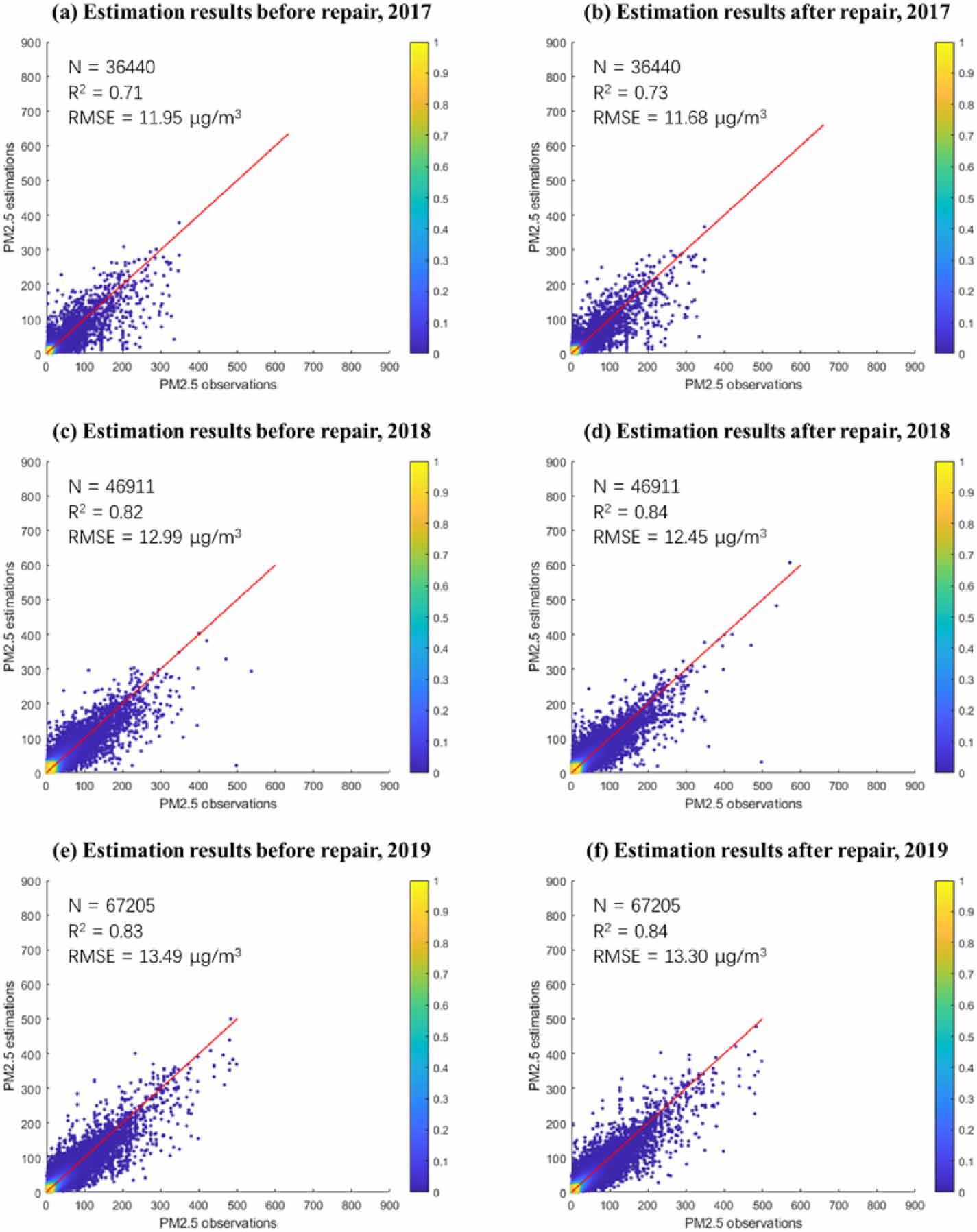
4. Conclusion
In this study, aiming at the problem of the missing values in the data of global air quality monitoring stations, we proposed a two-step hybrid model called ST-SILM to reconstruct the global PM2.5 monitoring data collected from OpenAQ from 2017 to 2019. In the proposed model, SES-IDW and LSTM were used in the 1st step and the 2nd step respectively to achieve spatio-temporal data reconstruction. We carried out the simulation experiment and the real experiment respectively, and the experiments proved that the proposed method showed its robustness and stability under the condition of increasing missing rate. At the same time, we applied the reconstructed data to remote sensing estimation of PM2.5. The results were better than those of the original observed data, proving the validity and reliability of the reconstructed data.
The method proposed in this paper has achieved satisfactory results. However, due to the limitation of spatio-temporal dependence, the PM2.5 concentration data from global air quality monitoring data cannot be completely repaired at present. Moreover, we underestimate peak pollution episodes because they are hard to learn. In the future, we will strive to break these limitations and achieve more comprehensive and higher quality reconstruction of global monitoring data. In addition, the application of the reconstructed data will be the direction of our further research. It is a common problem that the application of data cannot achieve good performance when the monitoring stations are far away from each other. Therefore, we will also construct virtual PM2.5 monitoring stations in the future work to densify sites and make the data application obtain better performance.
Acknowledgments
This work was supported in part by the National Natural Science Foundation of China (No. 41922008) and the Hubei Science Foundation for Distinguished Young Scholars (No. 2020CFA051). The authors would like to express gratitude to the OpenAQ platform for collecting global PM2.5 mass concentration data.
Conflict of interest
The authors declare no competing financial interests.