


Abstract
Current global-scale models of water resources do not generally represent groundwater lateral flows and groundwater–surface water interactions. But, models that do represent groundwater in more detail are becoming available and this raises the question of how estimates of water flow, availability, and impacts might change compared to previous global estimates. In this study, we provide the first global quantification of cell-to-cell groundwater flow (GWF) using a high-resolution global-scale GWF model and compare estimated impacts of groundwater pumping using two model setups: (a) with and (b) without including cell-to-cell GWFs and realistic simulation of groundwater–surface water interactions at the global scale (simulated over 1960–2010). Results show that 40% of the land–surface cell-to-cell flows are a notable part of the cell's water budget and that globally large differences in the impact of groundwater pumping are estimatd between the two runs. Globally, simulated groundwater discharge to rivers and streams increased by a factor of 1.2–2.2 when GWFs and interactions between groundwater and surface water were included. For eight heavily pumped aquifers, estimates of groundwater depletion decrease by a factor of 1.7–22. Furthermore, our results show that GWFs and interactions between groundwater and surface water contribute to the volume of groundwater that can be pumped without causing notable changes in storage. However, in approximately 40% of the world's watersheds where groundwater is used, groundwater is being pumped notably at the expense of river flow, and in 15% of the area globally depletion is increased as a result of nearby groundwater pumping. Evaluation of the model results showed that when groundwater lateral flows and groundwater–-surface water interactions were taken into account, the indirect observations of groundwater depletion and groundwater discharge were mimicked much better than when these fluxes were not included. Based on these findings, we suggest that including GWFs in large-scale water resources assessments will benefit a realistic assessment of groundwater availability worldwide, the estimation of impacts associated with groundwater pumping, especially when one is interested in the feedback between groundwater use and groundwater and surface water availability, and the impacts of current and future groundwater uses on the hydrological system.
Export citation and abstract BibTeX RIS

Original content from this work may be used under the terms of the Creative Commons Attribution 4.0 license. Any further distribution of this work must maintain attribution to the author(s) and the title of the work, journal citation and DOI.
1. Introduction
Groundwater is the largest available freshwater resource on Earth and is a critical supply for human systems and the environment. Groundwater is a major contributor to flow in many rivers and streams and has a strong influence on river and wetland habitats and ecosystems [1–3]. Groundwater contributes, directly and indirectly, to crop production via irrigation and by supporting soil moisture via capillary rise. Regional-scale studies have long emphasized the importance of including groundwater flow (GWF) for accurate model-based estimation of the available water in a catchment or aquifer, as well as for detailed assessments of the impact of water use on groundwater dynamics [e.g. 4, 5]. At the global scale this importance, i.e. any difference groundwater models might make to conventional model estimates, has not been substantially compared.
Although more accurate estimates of groundwater dynamics and the effects of groundwater use can be obtained from regional-scale models, because it can be assumed that regional-scale models use more accurate datasets, a better understanding of groundwater dynamics on a global scale is critical. Water demand and pressure on our groundwater resources continue to increase [6] and the effects of groundwater use extend beyond the regional scale. For example, groundwater interacts with climate through the modulation of surface energy and water distribution with long-term memory [e.g. 7–9]. For example, capillary rise from groundwater supports soil moisture and therewith evapotranspiration fluxes [10]. However, the broader temporal and spatial scales of the interaction between climate and groundwater remain partly unresolved [11]. Furthermore, lateral GWFs crossing catchment boundaries support water availability in receiving catchments or aquifers, and therewith support river low flows and groundwater availability in these receiving catchments and aquifers [1, 12]. This inter-basin GWF also means that upstream groundwater uses will impact downstream groundwater and surface water availability. Additionally, groundwater plays an important role in the global food-water-energy nexus and virtual groundwater trades are increasing at the global scale [13]. This means, for example, that a change in groundwater availability for crop production will directly impact regional and global food security. Lastly, regional approaches generally focus on important aquifer systems or regions where the negative impact of groundwater use is already experienced and are in general biased to regions where data of, for example, the subsurface is available. Thus, only a limited portion of the landmass and population is currently covered by regional-scale studies and many other parts that may be important for processes like surface water–groundwater exchange and evapotranspiration and that might experience negative impacts of groundwater pumping in the future, are either not covered or estimates (and hence globally available indices) may not be comparable due to different underlying data and methods.
Despite the importance of GWF as part of the environmental system, GWFs and exchanges of groundwater to surface water and soil moisture are represented as simple conceptual models or are even ignored, in most current global-scale hydrological models and water resources assessments [14]. Incorporating groundwater processes into global-scale simulations is particularly challenging because of the lack of robust subsurface data [15, 16], that are needed to realistically simulate groundwater heads and groundwater dynamics [e.g. 1, 12, 17], and the increasing computational times when more complexity is added (for example, by adding the simulation of GWF) [12, 17, 18]. Another reason that groundwater processes are often not included is that at the usual timescales considered within large scale hydrological models (i.e. from season to years), the amount of lateral flow across cell boundaries is assumed to be small compared to the vertical exchange between groundwater and the overlying soil through recharge, evaporation and capillary rise [19, 20]. Furthermore, often spatial scales of most current models are coarse (typically approximately 50 × 50 km) which makes cell-to-cell flow less relevant compared to vertical fluxes across the various climate and hydrogeological settings globally [21].
However, as there is a tendency to move to higher spatial resolutions (typically 10 × 10 km and finer) to improve regional accuracy of global-scale models, GWFs crossing cell boundaries will become more important compared to vertical fluxes [12, 21]. Furthermore, to understand the impact of groundwater pumping on streamflow, exchanges between groundwater and surface water have to be simulated. Without the simulation of groundwater heads, it becomes mathematically difficult to estimate realistically groundwater drainage and river infiltration at a global scale [12]. The integration of GWFs and the interactions of groundwater to surface water and soil moisture in large-scale hydrological models will improve current estimates of groundwater and surface water availability and will enhance our understanding of the current and future impacts of groundwater pumping on freshwater availability, environment, and soil moisture. The latter affects crop production and evapotranspiration fluxes.
In this study, we provide the first global quantification of cell-to-cell GWF using a high-resolution GWF and the contribution of this flow to groundwater availability for pumping and streamflow. We compared the model results of two model setups: (a) including GWF and (b) without GWF. Both models were run over the period 1960–2010. The results show for which conditions (i.e. hydrogeological, climatic, and human impact) GWF are most important to be included to obtain accurate estimates of the current and future impacts of groundwater pumping. The novelty of this research is that, with the GWF model and the comparison between the two model runs, we can provide an initial estimate of what proportion of the pumped groundwater comes either from the groundwater availability of adjacent cells or from streamflow.
2. Methods
2.1. Global-scale groundwater and surface water model
In this study, we used two model setups of the physically-based hydrological and water resources model PCR-GLOBWB [3, 22]. The model integrates human activities, including water use and reservoir regulation, into hydrology at high resolution (i.e. 5 arcminutes) at a daily time step. A summarized description is given here, a more detailed description of the model setup, model structure, and coupled modules is given in the supplementary information (SI) (available online at stacks.iop.org/ERL/17/044020/mmedia).
The model simulates for every grid cell and for every timestep the water storage in two vertical stacked soil layers and an underlying groundwater layer, as well as the water exchange between the layers (infiltration, percolation, and capillary rise) and between the top layer and the atmosphere (rainfall, evapotranspiration, and snowmelt) (see figure 1(a)) and solves the water balance. The model also calculates canopy interception and snow storage. Runoff, generated by snowmelt, surface runoff, interflow, and groundwater discharge, is routed (using kinematic wave routing) across the river network to the oceans and lakes.
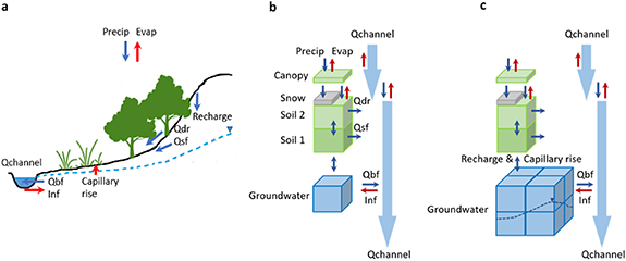
Figure 1. Model schematizations. (a) Conceptualization of the model setup, specifically illustrating the interactions between groundwater, surface water, and soil moisture. (b) Model conceptualization of PCR-GLOBWB (i.e. no-GWF setup). (c) Model conceptualization of PCR-GLOBWB-MF (i.e. GWF setup). Precip: precipitation, Evap: evapo(trans)piration, Qdr: overland flow, Qsf: sub-surface flow, Qbf: groundwater baseflow, Inf: river infiltration, Qchannel: river discharge.
Download figure:
Standard image High-resolution imageWe compared results using two versions of the model: (a) one where groundwater is represented as a linear reservoir and GWF between grid cells are ignored and groundwater–surface water and groundwater–soil moisture interactions are simulated very simplistically (figure 1(b), e.g. [22]) and (b) one where the linear reservoir is replaced by a two-layered GWF model (based on MODFLOW [23]), simulating groundwater heads, lateral GWFs, and head-dependent interactions between groundwater and surface water and groundwater and soil moisture (figure 1(c) [12, 24]). This model version is described in previous publications as PCR-GLOBWB-MF [3]. From here on we will call the first version of the model 'no GroundWater Flow' (no-GWF) and the second version 'GWF'. The GWF model is currently one-of-a-kind [3] and is unique in its parameterization of confined and unconfined aquifers at the global scale, needed to realistically simulate the impact of groundwater pumping on the groundwater system [12], and its integrated coupling to surface water and soil moisture estimated by the hydrological model [3].
Water demands for irrigation, industries, households, and livestock were estimated at the grid cell resolution [25]. The water abstractions and allocation of demands are calculated using a dynamic allocation scheme [26]. Total water demands were met from three resources, namely from surface water, groundwater, or desalinated water (figure S1(c)).
Both models are forced with spatial daily fields of precipitation, temperature, and reference potential evaporation over the period 1960–2010 [22].
2.2. Quantifying groundwater lateral flows
In the GWF model, GWF between grid cells is calculated and is head- and conductance-dependent [27]. First, we analysed under which conditions (i.e. climatological and subsurface parameterization) cell-to-cell GWFs are most significant. To exclude the impact of groundwater use on cell-to-cell GWFs we estimated this flux for naturalized conditions, i.e. excluding human water use.
Net GWF, L, was estimated from the water balance of each cells as:

R is groundwater recharge (positive sign) or capillary rise (negative sign), Q is groundwater drainage (negative sign) or river infiltration (positive sign) (Qbf or Inf in figure 1 respectively), and S is the change in groundwater storage. Net 'exporters' transport water to the adjacent downstream cells, while net 'importers' import water from the adjacent upstream cells. We classified the contribution of L to the groundwater budget of a cell as notable when L exceeds 10% of cells recharge or a minimum of 10 mm yr−1 (following the definition of significant GWF used by [21]). L is estimated and averaged over the period 1960–2010.
2.3. Evaluation of the role of groundwater lateral flows
Second, we evaluated differences between the two model setups regarding the estimated impacts of groundwater use. Specifically, we compared estimated groundwater depletion and groundwater discharge to rivers and streams.
2.3.1. Comparing groundwater depletion
Groundwater demand is an input to the model (figure S2) and will be pumped from surface water or groundwater resources. Groundwater recharge is estimated by the model as infiltrated precipitation reaching the groundwater (figure S4). When groundwater is abstracted according to this demand at rates higher than infiltration from precipitation (i.e. groundwater recharge) or rivers, groundwater levels drop, and groundwater is depleted [28, 29]. In the no-GWF run groundwater recharge in the cell is available for abstraction. If the groundwater demand and hence abstraction is smaller than the recharge, part of the recharge will satisfy water demands and part will be discharged to the river. If groundwater demands are larger than recharge the deficit between recharge and demand is estimated as groundwater depletion and groundwater discharge becomes zero. As a metric of analysis, the estimated groundwater depletion of the no-GWF run is accumulated over the period 1960–2010. Similar methodologies have been used in previously published research [30, 31]. In the GWF model setup, GWD is calculated from the simulated head decline and using aquifer storage coefficients (using data of GLHYMPSE2.0 [12, 15]).
The difference between the two model setups is evaluated by calculating the fraction of increase or decrease of the estimated GWD. This fraction, fGWD, is calculated as:

where GWDno-GWF and GWDGWF are the estimated GWD for the no-GWF and GWF model setups respectively. If fGWD is larger than 1, the depletion estimate is largest when lateral flows are not included. If fGWD is smaller than 1, the depletion estimate is largest when GWFs are included. If fGWD is 1, GWD did not differ The fraction is calculated at the cell level and as a metric for analysis, the average fraction was estimated over the aquifer area for eight heavily pumped aquifer systems around the world.
2.3.2. Comparing groundwater discharge
GWF contributes to river flow via groundwater drainage. In particular, during low flow conditions, GWFs support river low flows in general. On the other hand, when groundwater levels drop below river levels, groundwater discharges decrease and could eventually completely stop or turn around, becoming river infiltration [3, 29].
In the no-GWF model setup, groundwater–surface water interactions, either groundwater drainage or river infiltration (Q), are calculated as the deficit between groundwater recharge and storage change. In the GWF model setup, Q is simulated as a head-dependent flux including riverbed resistance [3].
The difference in estimated Q is evaluated by calculating the fraction of increase or decrease in estimated Q. This fraction, fQ , is calculated as:

where Qno-GWF and QGWF are the estimated Q for the no-GWF and GWF model setups respectively. If fQ is larger than 1, the estimated groundwater discharge is larger when lateral flows are not included. If fQ is smaller than 1, the estimated groundwater discharge is larger when GWFs are included. If fQ is 1, Q did not differ. It should be noted that for the no-GWF model setup only groundwater drainage is estimated, whereas in the GWF model setup also river infiltration can occur. The fraction fQ was estimated at the grid-cell resolution.
3. Results
3.1. Groundwater lateral flow
Over approximately 40% of the land surface net GWF, L, contributes notably to the groundwater availability in the cell; approximately 60% of these cells are 'groundwater exporters', transporting water to adjacent downstream cells, and 40% are 'groundwater importers', receiving groundwater from adjacent upstream cells. Regions that stand out as groundwater exporters are the globally wettest regions, for example, the Amazon, western Europe, Southeast Asia, including steep coastal regions, such as in Norway and British Columbia (Canada) (figure 2). Regions of groundwater import can, for example, be found for drier climatic regions such as the High Plains aquifer and Central Valley (USA), the Indus river basin, and the alluvial plains of South America (i.e. Gran Chaco).
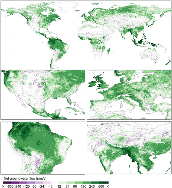
Figure 2. Estimated net groundwater flow for naturalized conditions averaged over 1960–2010 at the grid-cell level. The purple colours indicate net inflow, the green colours indicate net outflow.
Download figure:
Standard image High-resolution imageL is dominantly driven by groundwater recharge (R), as seen from the spatial distribution and magnitudes of L that highly correlate to estimated R (figures 2 and S3) and from the histogram (figure 3(a)). The histogram (figure 3(a)) shows that when recharge rates are low (<60 mm yr−1) L fluxes are small and slightly skewed towards import. When R rates are higher (60–120 mm yr−1) L fluxes get larger and slightly skewed towards export. For the highest R rates (>120 mm yr−1) groundwater export is dominant. Other drivers that have an impact on L are subsurface permeability (logk, figure S2) and depth to the water table (wtd, figure S4). The histogram of figure 3(b) shows that for low logk (−16 to −14 m2, e.g. siliciclastic sedimentary or crystalline rocks [15]) L fluxes are small and slightly skewed towards import. For higher logk (−14 to −12 m2, e.g. fine grained-, unconsolidated rocks [15]) L fluxes increase without skew. For the highest permeabilities (−12 to −10 m2 e.g. course grained unconsolidated rocks [15]) L fluxes are small again. The histogram of figure 3(c) shows that for shallow wtd (<10 m) the range of L fluxes is covered with a slight skew towards export. When wtd gets deeper (10–100 m) L fluxes get slightly smaller and skew towards import. For the deepest wtd (100 m and deeper) groundwater export is dominant.
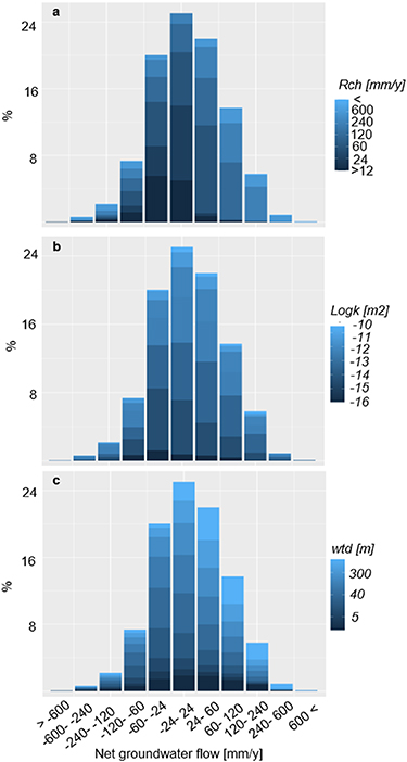
Figure 3. Histograms of net groundwater flow. Each bar in the histogram is clustered based on classified (a) estimated groundwater recharge, (b) estimated water table depths, and (c) permeability values.
Download figure:
Standard image High-resolution image3.2. Difference in groundwater depletion
The differences in estimated groundwater depletion between the two model setups are large (figure 4). For 85% of cells where groundwater abstraction takes place, groundwater depletion is higher when groundwater lateral flows are not included; for 15% of the cells, groundwater depletion is lower without including lateral flows. Differences are highest for regions where groundwater demands are high. For some aquifers where groundwater is used extensively, fGWD varies from 1.7 to 22 (for the High Plains aquifer system and the North China Plains respectively) (figure 4, table 1). Regions where estimated depletion is significantly lower when GWFs are not included are much more fragmented and can be found, for example, for parts of the High Plains aquifer (USA), and parts of India.
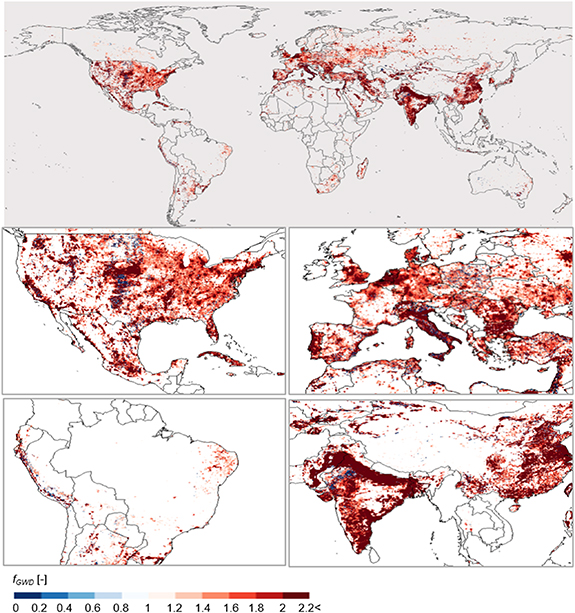
Figure 4. Estimated fraction fGWD at the cell level. The blue colours indicate a lower estimated groundwater depletion when groundwater flows are not included, the red colours indicate a higher estimated groundwater depletion when groundwater flows are not included.
Download figure:
Standard image High-resolution imageTable 1. Estimated groundwater depletion for eight intensively pumped aquifers and globally, compared to the literature. The pumping rates presented here are averaged values over the period 1960–2010.
| This study | Comparison | ||||||
|---|---|---|---|---|---|---|---|
| Aquifer | Aquifer size a (km2) | Averaged total groundwater abstraction per year (km3 yr−1 over 1960–2010) | GWDGWF (km3) | GWDno-GWF (km3) | FGWD | GWD (km3) | Reference |
| Central Valley | 64 300 | 10 | 94 | 340 | 3.6 | 98 | [33] |
| 75 | [36] | ||||||
| High Plains | 490 000 | 16 | 331 | 588 | 1.7 | 277 | [33] |
| 340 | [36] | ||||||
| Upper Ganges | 475 000 | 170 | 560 | 3550 | 6.3 | 16 b | [35] |
| Lower Ganges | 465 000 | 72 | −60 | 1220 | 20 | ||
| North China Plains | 228 000 | 34 | 38 | 862 | 22 | 178 | [33] |
| Western Mexico | 207 000 | 4 | 14 | 125 | 8 | ||
| Arabian | 1900 000 | 7 | 111 | 250 | 2.2 | ||
| Persian | 393 000 | 9 | 28 | 298 | 10 | ||
| Global | 730 | 2000 | 12 000 | 5 | 18 000 | [30] | |
| 2000 | [33] | ||||||
a Aquifer polygons were used from WHYMAP (available from http://whymap.org) and gridded at the grid cell resolution to estimate aquifer size. b Upper and lower Ganges.
3.3. The difference in groundwater discharge
Differences in estimated groundwater discharge between the two model setups show clear patterns as well (figure 5). For 65% of cells where groundwater discharge is estimated, this flux decreased when groundwater lateral flows were not included; for 35% of the cells, groundwater discharge increased without groundwater lateral flows.

Figure 5. Estimated fraction, fQ , at the cell level. The blue colours indicate an increase in estimated groundwater discharge when groundwater flows are not included. The red colours indicate a decrease in estimated groundwater discharge when groundwater flows are not included.
Download figure:
Standard image High-resolution imageFrom figure 5, the larger rivers and streams can be identified as increased or decreased groundwater discharge features. Regions where groundwater discharges decreased without accounting for groundwater lateral flow and groundwater–surface water interactions, are, for example, the eastern part of the USA, south-western Europe, and Southeast Asia. Also, a strong decrease in groundwater discharge is found for some intensively irrigated regions, such as the Mississippi Embayment, the Ganges river basin, and part of the North China Plains. Regions where we see an increase in groundwater discharge, are, for example, the plateau regions in Asia and the region south of the Sahel, and more concentrated 'hotspots', like Southern Central Valley, upper Kansas River, and rivers in Southern Spain.
3.4. Model evaluation
Detailed model evaluation (both for the no-GWF and GWF versions) on groundwater recharge, water demands, and allocation, and water table depths was done in previous studies [12, 22, 24, 31] as well as detailed model sensitivity tests varying subsurface parameter settings, and boundary conditions [3]. Here we provide additional validation specifically relevant to the depletion and groundwater discharge that we compared in this study.
Direct observations of this cell-to-cell GWF are unavailable at the global scale. To evaluate the model results we compared our estimates of groundwater discharge (Q) to two selected regional data sources available from previous studies, (a) indirect observations obtained by baseflow separation of streamflow observations of several catchments in Kansas; to (b) simulated groundwater discharges of catchment scale calibrated models. For the first, streamflow data of 50 stations in Kansas, USA, where groundwater pumping is the dominant water use were used [3]. For the latter, we used modelled groundwater discharges for several calibrated catchment-scale models [3] spread over different continents and climate zones of the world. As these models are calibrated, it is assumed their estimated groundwater discharge is as accurate as possible.
The simulated Q of both model runs is compared to the separated observed baseflow Qb and the simulated Qs of the calibrated models (figure 6). Figure 6 shows that the simulated Q of the GWF run better fits the indirectly observed and calibrated Qs than the results of the no-GWF run (i.e. R2 of 0.99 and 0.82 respectively). In general Qs of the no-GWF are all underestimated. We acknowledge that this model evaluation is limited to a few locations of observations, only providing the first glance of model performance of estimated groundwater discharge. However, currently, the availability of datasets of (indirect) observations is very limited [3, 4, 32].

Figure 6. Evaluation groundwater discharge. Comparing simulated groundwater discharge to observed baseflows (Kansas) and calibrated estimates (indicated stations). The dashed line represents the 1:1 line.
Download figure:
Standard image High-resolution image
Further model evaluation is focused on estimated groundwater depletion. Table 1 compares this study's depletion estimates for several large, intensively pumped, aquifer systems to previously published estimates using modelling approaches similar to our no-GWF approach [30, 31] and methods that interpolated observations [33–35]. The estimated global depletion (over 1960–2010) ranges between 18.000 km3 [30] and 2.000 km3 [33] depending on the approach used. This study's estimated groundwater depletion falls between this range. As expected, the difference between the two model runs at global and aquifer scales is large and GWF estimates match the interpolated results best. This illustrates that, when GWFs and groundwater–surface water interactions are included, estimated groundwater availability and impacts of groundwater pumping are simulated more accurately than when GWFs and groundwater–surface water interactions are not accounted for. This is in line with the conclusion drawn in [36] that current global models (without GWFs) are unable to predict accurately long-term trends on terrestrial water storages compared to satellite observations from GRACE. Similar conclusions were drawn at the aquifer scale, for example, in [29, 35], where the missing GWF and groundwater–surface water interactions are identified as the main driver of uncertainty in their groundwater depletion estimates. Also, for example, [5] already stated that increased capture caused by groundwater pumping will help to minimize the resulting head decline, and thus groundwater depletion; although at the expense of river discharge [3]. This conclusion is confirmed by our findings. We estimated that in approximately 40% of the world's watersheds where groundwater is used, groundwater is being pumped notably at the expense of river flow.
On the other hand, for the Upper Ganges and North China plain simulated groundwater depletion of the GWF run are much higher than interpolated depletion estimates and indicate model uncertainties in this study are still large, at least for some regions of the world. This uncertainty is expected to increase when groundwater depletion estimates are evaluated at smaller scales (e.g. cell level) driven by uncertainties in simulated groundwater recharge, aquifer parameterization, and estimated water demands.
4. Discussion: importance of groundwater lateral flows in large-scale water resources assessments
Our results showed L is dominantly driven by groundwater recharge (figure 3). Generally, groundwater export is simulated for moist regions with moderate relief, where shallow water tables are connected to the local streams, such as in Europe and Southeast Asia. Other regions that stand out are steep coastal areas, such as Norway and British Columbia, and, to some extent, mountain regions, such as the Appalachians, where GWFs into local aquifer systems connected rivers and streams at a higher elevation. Generally, groundwater import is simulated for drier regions of the world where water tables are deep, and where elevation differences are larger, such as for the High Plains aquifer, Central Valley, Indus river basin, and the high lands of South America (figures 2–5).
Including groundwater lateral flow and groundwater–surface water interactions has clear effects on the estimated impact of groundwater use at the global scale. Results showed that cell-to-cell GWF redistributes groundwater recharge and supports groundwater availability for river flow and pumping in receiving cells. The magnitude of groundwater pumping can be identified as the main driver for the difference in estimated impacts when comparing the two model setups. For example, in regions where significant groundwater export is simulated but where groundwater demands are low, such as for the Amazon, a large part of Canada, and Russia, simulating GWF and groundwater–surface water interactions did not change the estimated groundwater depletion or groundwater discharge much (figure 5). Also, when comparing groundwater discharges, it stands out that in the no-GWF run more groundwater is drained at higher elevations compared to the GWF run (figure 5). In the no-GWF run, all recharge not used in the cell will be drained to the local drainage. In the GWF, for the higher elevated regions, groundwater tables are generally deeper and disconnected from the local drainage resulting in groundwater being transported further downstream, following long GWF paths. The increase in groundwater availability supported by cell-to-cell GWF results in a strikingly different estimate of groundwater depletion worldwide (figure 4). In particular, the intensively irrigated regions around the world stand out, for example, the Indus river basin, Ganges river basin, and the Mississippi Embayment. For these regions, shallow water tables that are connected to the local drainage are supported by GWFs from higher elevated regions. A similar conclusion can be drawn for the drier regions of the world, such as the High Plains aquifer and Central Valley. However, groundwater levels in these aquifers are deeper and connected to the regional drainage only. GWF from higher elevations helps to maintain water levels here as well, and support groundwater availability and regional drainage. But, groundwater levels in these drier regions are more sensitive to storage changes [12] compared to the wetter regions (e.g. Mississippi Embayment, Ganges river basin). Also, for the drier regions, groundwater depletion is reduced when GWFs are included, but for some parts of the aquifer, at the expense of water availability in the adjacent cell when groundwater levels in a cell drop due to pumping in a neighbouring cell (figure 4).
Based on the findings of this study, we suggest GWFs should be included for a realistic and in-depth assessment of groundwater availability worldwide and the estimation of impacts related to groundwater use. Our results show that the cell-to-cell GWF is as important as vertical fluxes, if not more important, for many regions of the world where groundwater is used, given the large differences in estimated groundwater depletion and groundwater discharge. Furthermore, the impact of groundwater abstractions extends beyond the grid-cell resolution when lateral GWFs are accounted for. This impact is seen both as an increase in depletion or river infiltration. These findings confirm and extend previous conclusions drawn for the US [1, 38] and globally [21]. These previous studies used water balance approaches, providing steady-state results, and did not include human water uses but identified groundwater use as the most important driver for biases in the results. Also, when one is also interested in the feedbacks between groundwater use and water availability in other parts of the Earth's system, interactions between groundwater and other parts of the system should be included. For example, GWFs and interactions should be included to quantify the contribution of groundwater to environmentally critical streamflow, which is variable over the season [3, 25]. Or, to quantify groundwaters' indirect contribution to crop production by supporting soil moisture [39], or to quantify groundwaters' support to evapotranspiration globally [10, 11]. Additionally, especially for regions where detailed regional-scale GWF models are not available, the results of a global-scale model can provide a first-order estimate of the current state of the groundwater system and expected impacts of groundwater use.
Model uncertainties exist. Drivers of model uncertainty are climate input, water demand, and water use inputs and assumptions, model parameterization, and the parameterization of boundary conditions. Extensive model uncertainty tests were done in previous studies. From these previous studies and the model evaluation done in this study, it is clear that at the global-scale, model uncertainty varies regionally and it is expected that this will improve when more accurate regional data becomes available worldwide and when some current model conceptualizations are improved [3, 14, 16, 20]. Therefore, future efforts in model development should focus on extending and improving globally available datasets of, for example, the subsurface or water demands, to be used for model parameterization and evaluation, and GWFs should be simulated globally, especially when moving to finer resolutions [4, 16].
5. Conclusion
The impact of GWFs and groundwater–surface water interactions is significant for many regions of the world. This study showed estimated cell-to-cell GWF using a global-scale two-layered GWF model for the first time, allowing us to conclude that cell-to-cell flow plays an important role in redistributing groundwater recharge spatially. This redistribution makes significant contributions to freshwater availability at a larger scale, especially for regions where groundwater demands are high. Such regions include irrigated regions around the world where thick permeable aquifers are present and where groundwater recharged at higher elevations flows to and supports water availability in lowland aquifer systems. Our study showed, at the global scale, that including groundwater lateral flows results in lower estimated depletion from groundwater pumping on groundwater storage, however, possibly at the expense of higher reductions in river discharge. The two impacts, therefore, need to be estimated together and considered more thoroughly in future assessments.
The insights obtained from this study can be the starting point for further deepening our knowledge of the groundwater system worldwide and its sensitivity to changes in storage, either caused by human water use or climate change. Especially for regions where detailed regional-scale models do not exist, the results of a global-scale groundwater model can give an improved first-order estimate of current and expected impacts of groundwater use than currently available. Furthermore, the simulation of the interaction of groundwater with streamflow and soil moisture will allow a further global-scale analysis of the contribution of groundwater to evapotranspiration and crop production.
Acknowledgments
The authors acknowledge support by the state of Baden-Württemberg through bwHPC and the German Research Foundation (DFG) through Grant No. INST 39/963-1 FUGG (bwForCluster NEMO).
Data availability statement
The data that support the findings of this study are openly available at the following URL/DOI: https://datacommons.cyverse.org/browse/iplant/home/shared/commons_repo/curated/DeGraaf_data_comparison_lateral_groundwater_flows_2022.