

Abstract
Elevation data are fundamental to many applications, especially in geosciences. The latest global elevation data contains forest and building artifacts that limit its usefulness for applications that require precise terrain heights, in particular flood simulation. Here, we use machine learning to remove buildings and forests from the Copernicus Digital Elevation Model to produce, for the first time, a global map of elevation with buildings and forests removed at 1 arc second (∼30 m) grid spacing. We train our correction algorithm on a unique set of reference elevation data from 12 countries, covering a wide range of climate zones and urban extents. Hence, this approach has much wider applicability compared to previous DEMs trained on data from a single country. Our method reduces mean absolute vertical error in built-up areas from 1.61 to 1.12 m, and in forests from 5.15 to 2.88 m. The new elevation map is more accurate than existing global elevation maps and will strengthen applications and models where high quality global terrain information is required.
Export citation and abstract BibTeX RIS

Original content from this work may be used under the terms of the Creative Commons Attribution 4.0 license. Any further distribution of this work must maintain attribution to the author(s) and the title of the work, journal citation and DOI.
1. Introduction
Topographic information, described here as digital elevation models (DEMs), are crucial inputs for a diverse range of applications in fields such as demography [1], ecology [2, 3], geomorphology [4, 5], glaciology [6, 7], hydrology [8–10], soil science [11] and volcanology [12, 13]. At the global scale, elevations are measured from space using near-infrared, radar and visible sensors, and then georectified and stored in a gridded storage structure. DEMs exist at the global scale, or near-global scale, at 3 arc second (∼90 m), and more recently 1 arc second (∼30 m) grid spacing. The global DEMs at 3 arc second grid spacing include the widely used Shuttle Radar Topography Mission (SRTM) [14], as well as MERIT [15], TanDEM-X 90 [16, 17] and Copernicus GLO-90. At 1 arc second, products include ASTER GDEM (v3) [18], ALOS World3D AW3D30 (v3.2) [19], SRTM [14], NASADEM [20] and most recently Copernicus GLO-30 [21] (herewith referred to as COPDEM30).
The acquisition period, sensor type, processing, post-processing and geographical extent varies between DEMs [22]. As a result, accuracy, and therefore suitability, for a given application varies. COPDEM30, and the underlying TanDEM-X data, is the most recent and accurate global DEM [23–25]. COPDEM30 can accurately resolve most features, with Guth and Geoffroy [25] going as far to say COPDEM30 should become the 'gold standard' for global DEMs. Hence COPDEM30 was chosen as the basis of this work for producing a global bare-earth DEM.
DEMs can be broadly separated into digital surface models (DSM), which measures the upper surface of trees, buildings and other man-made features, and digital terrain models (DTMs) which measures the elevation of the ground surface, or the 'bare-earth' [26]. Each DEM has a different abstraction of the real surface. The presence of tree and building bias in DEMs is problematic in some applications, particularly in hydrology, where artifacts in the DEM can act as dams that change overland flow pathways. It is up to the user to decide which abstraction is best for their application, and they can be guided by the numerous accuracy assessment studies [27–30].
DEMs at the global scale fall towards the DSM end of the DSM-DTM spectrum. The MERIT DEM is an exception, as tree height bias has been removed, along with absolute bias, speckle noise and striping. Therefore, MERIT DEM is closer to a DTM than other global DEMs. Other examples of tree height bias being removed are in the quasi global CoastalDEM [31] and vegetation removal from SRTM of O'Loughlin et al [32], Zhao et al [33] or Magruder et al [34]. Although there have been promising recent developments [35], the removal of buildings from MERIT at the global scale has not yet occurred, and thus MERIT cannot be considered completely as a DTM. With the rich amount of auxiliary data related to global building and forest coverage now available, there is increasing potential to utilise machine learning techniques to remove trees [31], buildings [35, 36] or both [37–39], although to date these studies are limited to the local or quasi global scale. Machine learning allows us to 'learn by example' by building empirical models from the data alone and is particularly well suited to non-linear settings [40].
Using machine learning techniques, we remove building and tree height bias from COPDEM30 to create a new data-set called FABDEM (Forest And Buildings removed Copernicus DEM). The new data-set is available between 60∘ S and 80∘ N at 1 arc second (∼30 m) grid spacing and is the first global DEM to remove both trees and buildings. We validate against reference elevation data and compare it to other global DEMs. Many applications where representation of the terrain is important will benefit from the improved resolution and accuracy of FABDEM compared to existing global DEMs. This is especially true of flood inundation modelling, where the terrain is a key determinant of water flows and hence locations of flooding.
2. Methods
2.1. Random forest regression
This study uses random forest regression models, which are popular in similar large-scale applications in remote sensing [41]. Random forest regression has recently been used for forest correction of SRTM [42], urban correction of MERIT [35] and correcting SRTM in New Zealand [39]. However to date, correction of DEMs using random forest models has not been utilised at the global scale.
In the preliminary stage of this study, we assessed generalized linear models (GLMs) and generalized additive models (GAM). Neural networks have also been used successfully at the quasi-global scale for the CoastalDEM [31] and at the local scale [37–39]. We found random forests to be accurate, computationally efficient and robust, hence an appropriate choice for this application.
Random forests take a 'divide and conquer' approach by combining outcomes from a sequence of regression decision trees, and are particularly popular as they have few parameters to tune, are robust to over-fitting and are robust to small and large data-sets [43, 44]. Accuracy is measured by 'out of bag error' which estimates error computed on reference data set aside prior to building the random forest model. In this study, 25% of the reference data are set aside for validation. We utilise a GPU accelerated random forest implementation in python which shows enhanced computational efficiency compared to CPU equivalents [45].
Once a machine learning algorithm is selected, the other key ingredients are a comprehensive reference data-set for training the model, and predictor variables. In machine learning, predictors or features are input variables used to predict the reference data or the target variable, hence predictors must be conceptually relatable to the application. Different predictors are used in the forest and buildings correction models, described further in sections 2.4 and 2.5.
2.2. Correction workflow
The workflow of producing FABDEM is shown in figure 1. This consists of three stages: (1) data preparation, consisting of processing predictor data and reference DEMs; (2) Random forest correction, done separately for forests and buildings removal and (3) post-processing, to merge the corrected DEMs, fill unrealistic pits and apply smoothing filters. Each step of the workflow is described below, as well as the data contributing towards the machine learning based correction.

Figure 1. Schematic of the workflow to create FABDEM. Data preparation is followed by the forest and building corrections, before merging the corrected surfaces and post-processing.
Download figure:
Standard image High-resolution image2.3. Data preparation
All data used in the FABDEM production were processed and regridded to the COPDEM30 grid (EPSG 4326 projection, at 1 arc second horizontal grid spacing). The predictor data and reference DEMs were then compiled into a tabular data format used by the random forest model.
Predictor data that were determined to be useful in estimating anomalies in the DSM associated with buildings and trees were chosen. The key data-sets describing forest height, forest cover and building footprints have a similar resolution (10–100 m) to COPDEM30, allowing them to provide information at the grid-cell level. Predictor variables are described in the respective sections on Forests and Buildings removal (2.4 and 2.5) and the full list of predictors are listed in supplementary table S1 (available online at stacks.iop.org/ERL/17/024016/mmedia).
An extensive search of LiDAR DTM data was carried out to select reference data for training the random forest algorithm. We specified that LiDAR data should have an accuracy of  1 m which comfortably adheres to the recommendation that reference data should be at least three times more accurate than the DEM [46]. A visual inspection of the data was initially implemented as a first quality check. LiDAR DTMs from 12 countries were selected to use in training the random forest algorithm, see supplementary table S2 for details of each data set. This reference data covers a wide range of climatic zones and urban areas, thus allowing us to use our approach at a global scale. A map showing spatial distribution of these data sets is included in supplementary figure S1. The reference DEMs were reprojected to the COPDEM30 horizontal grid and to the COPDEM30 vertical coordinates (EGM2008), using geoid models specifying the vertical datum used in each reference DTM.
2.4. Forest removal
We use a random forest model to predict the difference between COPDEM30 elevations and terrain elevations from a reference data (LiDAR) for forested regions. Therefore, variables are needed to estimate the height of the forest and the canopy coverage of the forest. The characteristic of the forest is important as the penetration of the radar signal used in COPDEM30 penetrates the tree canopy differently depending on the characteristics of the tree and the radar characteristics [47, 48].
The predictor data for forest height is taken from the Global Forest Canopy Height 2019 data-set [49]. Global Ecosystem Dynamics Investigation (GEDI) LiDAR data onboard the International Space Station [50] has been integrated with Landsat GLAD ARD [51] data to create an estimate of forest canopy height at 30 m grid spacing. Coverage is limited to the extent of GEDI footprint-based measurements, which are collected between 51.6∘ N and 51.6∘ S. A separate predictor variable, tree cover fraction from the Copernicus Global Land Service collection 3 epoch 2015 [52] was used to characterise canopy coverage of each 100 m cell globally. To decide where the regression model was applied, cells where both the forest height was greater than 3 m and tree cover was greater than 10% were considered forested for the vegetation correction algorithm below 52∘ N.
In regions outside the Global Forest Canopy Height 2019 data-set (above 52∘ N), we estimated canopy height using ICESat-2 L3A Land and Vegetation Height (version 4) ATL-08 data [53]. The 'h_canopy' and h_canopy_mean' variables were used, representing the top of canopy and mean canopy height respectively [54]. The ATL-08 terrain measurements have a reported bias of −0.07 to 0.18 m [55, 56]. ICESat-2 records with non missing-values over land were used. Additionally, records were discarded if h_canopy was greater than 50 m and for h_canopy values between 30–50 m, if the layer_flag was equal to 1. Values between ICESat-2 canopy height measurements were interpolated to increase the coverage of canopy height estimates. Cells with canopy coverage  from the Copernicus Global Land Service Collection were considered forested and used in the forest correction algorithm above 52∘ N.
Additional predictor variables for the machine learning model were created by applying several image processing tools implemented in WhiteboxTools [57]. These filters were applied to both the COPDEM30 elevations and the tree height data, to detect features such as edges, anomalies or variability that might be due to forests. For example, a sobel edge detector filter with a  window was applied, and an unsharp filter was applied to emphasize edges, while reducing noise. Filters computing the difference between gaussian filters of varying sizes were also computed. Lastly, a bilateral edge-preserving smoothing filter and gaussian filters to emphasize long-range variability were applied to the forest height variable only.
An overview of the data-sets used to train the model and their filtered versions are in table S1 of the supplementary material, and the number of samples per country of LiDAR data are in table S2.
2.5. Buildings removal
A separate random forest model was built to predict the differences between COPDEM30 elevation and terrain elevation from LiDAR for urban areas. Multiple predictor data-sets were used for building removal to characterise factors relating to building height, for example building footprints, population and socio-economic indicators. In their urban correction of MERIT DEM, Liu et al [35] reported limitations of the transferability of their model due to the relatively small training data-set being unable to capture the variability of buildings in urban areas, leading to overestimation particularly in smaller cities. Hence in this study, we use a range of independent data-sets to increase the applicability of our model.
Predictor data-sets include information on population density (WorldPop [58]), travel times [59], night-time lights [60], urban building footprints (World Settlement Footprint [61]), built-up areas per capita, GDP and average greenness (GHS-UCDB R2019A [62]). Further detail on these predictor variables is given in the supplementary text S2 and table S1.
Data on building footprints and density from OpenStreetMap were not used due to the lack of global consistency [63] and the low importance of the variable(s) in other location specific random forest based DEM correction studies [35, 39]. Log transformations were applied to population, GDP per area and travel times. As for the forest correction, filters (difference of gaussians, sobel and unsharp) were applied, but in this case to detect edges of urban areas or taller buildings in COPDEM30. The number of samples per LiDAR country for building removal are detailed in table S2.
2.6. Post processing
Correction surfaces simulated through random forest models for both forest and buildings were subtracted from COPDEM30 to get the terrain elevations. Therefore, as illustrated in figure 1, two intermediate layers were produced—COPDEM30 Building removed and COPDEM30 Forest removed. The COPDEM30 Building removed and COPDEM30 Forest removed layers were subsequently merged, taking the minimum value at each pixel. Locations adjacent to the COPDEM30 water-body mask (WBM), were handled separately, without buildings or forest removal being applied. This was to ensure that coastline/riverbank pixels were not overly lowered, but were kept consistent with the surrounding terrain. Locations underneath the WBM had no modifications made and are essentially identical to the COPDEM30 values.
Additional steps were applied to correct areas that had been corrected too much, or areas where pixels were noisy. Firstly, to remove artifacts outside building and forest corrected areas, pits up to 4 pixels in size were filled. In building and forest removed areas, large depressions were filled, but not higher than the original COPDEM30 (after filling small pits in the COPDEM30 of up to 100 pixels in size). Only pixels that had been adjusted (i.e. Building and Forested) were filled. Noise in the DEM was subsequently reduced by running an adaptive filter twice, and then a bilateral filter. An adaptive filter is effective at removing speckle noise [64], and was used in MERIT DEM [15]. A bilateral filter is an edge preserving smoothing filter [65] that preserves edges of features but reduces short-scale variation. These filters were implemented in WhiteBoxTools [57].
Further smoothing was done for pixels adjacent to the WBM, with a  pixel median filter applied to non-water pixels, with a subsequent single pit filling step. This step was necessary as we noted COPDEM30 contained incidences of pits. Finally, all smoothed sections of the DEM (values adjacent to WBM, WBM and all other land pixels) were combined to create FABDEM. Guidance of parameter selection for the filters are limited at the scale of global DEMs [66, 67], as studies predominantly focus on finer grid spacing LiDAR data [68–70]. Therefore, parameters were selected using an extensive trial and error approach.
3. Results and discussion
To demonstrate the utility of the FABDEM data-set we validate the DEM against reference elevation data, as well as comparing against other global DEMs. We use two sources of reference data. (1) LiDAR data from 12 countries (listed in supplementary table 2) and (2) ICESat best estimates of the ground terrain, randomly sampled from locations around the globe. Additionally, reference data over Florida, USA (not used in training) was obtained for a visual comparison.
We note here that the reference LiDAR data used for validation in section 3.2 are the same as the training data. A random sample of 1000 points per tile that contains LIDAR data were used for validation. These sampled points were taken from the whole reference LiDAR dataset. Similarly, the training data was randomly sampled from the reference dataset (see table S2 for details), so some of the validation points were also used for training. However, the ICESat elevation data are not used for training, and are evenly distributed across the globe, so give an independent estimate of errors across all terrain types.
Other global DEMs were also compared against FABDEM: the original COPDEM30, MERIT DEM [15], CoastalDEM [31] and NASADEM [20]. Particular focus is made of the comparison against MERIT DEM, as MERIT DEM has had errors from vegetation removed, and is thus most similar to FABDEM.
3.1. Split-sample validation
When building the random forest models, 75% of the data samples were used for training the models and 25% of the data samples were kept back and used for validation only. This approach is known as split-sample or out of bag validation, and is useful to ensure the model is not being over-fitted and has some applicability outside of the training set.
For the urban correction, the reference COPDEM30 data had a mean absolute error (MAE) of 1.72 m, which was reduced to 0.94 m for predictions on the training sample, while predictions on the validation sample had MAE of 1.35 m. For the forest model (south of 52∘ N), the split-sample validation results were: MAE of 7.2 m for the COPDEM30 data, MAE of 3.52 m in predictions on the training sample, and MAE of 6.55 m in predictions on the validation sample. Finally, for the boreal forest model (north of 52∘ N), the split-sample validation results were MAE of 3.77 m for COPDEM30 data, MAE of 1.72 m in predictions on the training sample, and MAE of 3.24 m in predictions on the validation sample.
In each case, the errors in the validation samples are greater than the training samples, but reduced compared to the COPDEM30 data. The results for the split-sample validations above are errors against reference data for the random forest model predictions before any post-processing is applied. So we validate separately on the final DEM after post-processing.
3.2. Global comparison
Figure 2 shows histograms of errors of FABDEM, COPDEM30 and MERIT DEM against reference data. Panels (a)–(c) show errors for urban, forest areas (south of 52∘ N) and boreal forest areas (north of 52∘ N) respectively. These consistently have lower errors in FABDEM compared to COPDEM30 and MERIT DEM, showing the benefit of both the newer COPDEM30 data-set compared to elevations based on SRTM, and the effectiveness of the forests and buildings correction applied for FABDEM. Table 1 presents some statistics corresponding to the histograms in figure 2. FABDEM has median errors close to 0 m, and the lowest errors in each of the statistics, showing a improvement on both COPDEM30 and MERIT DEM.

Figure 2. Histograms comparing FABDEM with COPDEM30 and MERIT DEM against reference data. 1000 grid cells are sampled per  tile containing reference data. Note that the reference data used here are the same data-set used for training the machine learning models, but are a different random sample.
Download figure:
Standard image High-resolution imageTable 1. Error statistics comparing COPDEM30, FABDEM and MERIT DEM against reference DEMs for each of the correction methods. Comparisons are only made for land cells where the FABDEM correction of the respective type was applied. ME is mean error, MAE is mean absolute error and RMSE is root mean squared error.
| Area | DEM | ME | MAE | RMSE | 90% Error | Error %  2 m 2 m |
|---|---|---|---|---|---|---|
| COPDEM30 | 0.86 | 1.61 | 2.87 | 3.54 | 74.77% | |
| Urban | FABDEM | −0.08 | 1.12 | 2.33 | 2.39 | 86.37% |
| MERIT DEM | 1.74 | 3.59 | 7.15 | 6.86 | 42.73% | |
| COPDEM30 | 2.93 | 5.15 | 7.98 | 12.51 | 35.52% | |
| Forest | FABDEM | 0.20 | 2.88 | 4.96 | 6.67 | 55.07% |
| MERIT DEM | 2.37 | 5.47 | 8.06 | 12.08 | 26.72% | |
| COPDEM30 | 0.72 | 3.49 | 7.73 | 9.64 | 62.46% | |
| Boreal Forest | FABDEM | −0.11 | 2.55 | 6.66 | 5.51 | 68.70% |
| MERIT DEM | 1.14 | 9.38 | 19.62 | 24.24 | 33.58% |
Figure 3 shows errors compared to ICESat-2 L3A Land and Vegetation Height (version 4) ATL-08 data [53]: for all land pixels (a) and over flood plains (b). Flood plains were delineated using the GFPLAIN250m data-set [71]. We use the ICESat-2 'h_te_best_fit' variable in this evaluation, which is the best estimate of terrain elevation [72, 73]. ICESat-2 ATL-08 canopy and ground surface data are processed in 100 m segments where a suitable number of photons are present, resulting in features not always being detected that are in the 1 arc second DEMs.

Figure 3. Histograms comparing FABDEM with COPDEM30 and MERIT DEM against ICESat2 'h_te_best_fit' elevations. 1000 samples are taken from each of 1900 randomly selected  tiles across the globe (10% of tiles). (a) Compares all land cells and (b) compares cells identified as flood plain in the GFPLAIN250m data-set [71].
Download figure:
Standard image High-resolution imageAs both non-urban and non-forested pixels (which are not corrected) are considered, the histogram of FABDEM and COPDEM30 are very similar, with both showing errors closer to 0 m compared to MERIT DEM. Table 2 presents some statistics corresponding to the histograms in figure 3, and some additional categories based on population density and forest canopy cover. The COPDEM30 and FABDEM distributions are centered around 0 m error, but have a relatively long tail. The MERIT DEM distribution is centered around 1 m error, which is reflected by the worst median error for floodplains, at 0.66 m, compared to −0.03 m of FABDEM. There are fewer large errors in MERIT DEM and FABDEM compared to COPDEM30, as reflected by the lower RMSE and 90% error values and higher % error  2 m values. Indeed, over floodplains, FABDEM and MERIT DEM have very similar error
  2 m at 80.42% and 80.19% respectively, with FABDEM having slightly better RMSE and 90% error values suggesting the tail of the error distribution is not quite as long as MERIT DEM. This is likely to be due to FABDEM having urban areas removed.
Table 2. Error statistics comparing COPDEM30, FABDEM and MERIT DEM against ICESat2 elevation data for land points, floodplain points (defined by the GFPLAIN250m data-set), canopy cover and population density. ME is mean error, MAE is mean absolute error and RMSE is root mean squared error.
| Cells | DEM | ME | MAE | RMSE | 90% error | Error %  2 m 2 m |
|---|---|---|---|---|---|---|
| COPDEM30 | 0.71 | 6.37 | 14.32 | 19.70 | 57.99% | |
| Land points | FABDEM | −0.07 | 3.41 | 11.13 | 8.85 | 67.50% |
| MERIT DEM | 0.81 | 4.81 | 13.13 | 12.55 | 60.90% | |
| COPDEM30 | 0.17 | 4.04 | 10.21 | 14.29 | 71.14% | |
| Floodplain | FABDEM | −0.03 | 2.03 | 7.87 | 4.90 | 80.42% |
| MERIT DEM | 0.66 | 2.35 | 8.04 | 5.61 | 80.19% | |
| COPDEM30 | 0.98 | 4.22 | 12.95 | 11.16 | 62.42% | |
Populated ( 5000 km2) 5000 km2) | FABDEM | 0.35 | 3.50 | 12.46 | 8.88 | 70.32% |
| MERIT DEM | 0.75 | 4.14 | 12.90 | 10.23 | 62.96% | |
| COPDEM30 | 1.90 | 4.99 | 14.33 | 12.73 | 50.90% | |
Populated ( 5000 km2) 5000 km2) | FABDEM | 0.19 | 3.94 | 13.75 | 9.90 | 61.31% |
| MERIT DEM | 0.85 | 4.35 | 14.16 | 11.72 | 59.04% | |
| COPDEM30 | 0.55 | 3.41 | 11.89 | 9.43 | 69.96% | |
| Canopy cover: 10%–50% | FABDEM | 0.20 | 2.92 | 11.53 | 7.59 | 75.96% |
| MERIT DEM | 0.71 | 3.84 | 12.74 | 9.60 | 68.57% | |
| COPDEM30 | 12.09 | 14.03 | 26.70 | 26.55 | 13.33% | |
Canopy cover:  50% 50% | FABDEM | 0.45 | 6.10 | 22.17 | 12.76 | 35.29% |
| MERIT DEM | 2.95 | 8.14 | 23.60 | 17.72 | 30.81% |
The spatial distribution of median biases in COPDEM30 and FABDEM compared to ICESat is shown in figure S2. This highlights the large scale biases in COPDEM which are removed in FABDEM. Regions do exist with biases remaining in FABDEM, including areas of steep terrain, however these areas also correspond to higher biases in ICESat [74].
In populated areas, FABDEM has the lowest median error, RMSE and 90% error, with the improvement over COPDEM30 most evident in the densest populated areas ( 5000 km2) where the median error of FABDEM is 0.19 m compared to 1.90 m in COPDEM30. The correction in forested areas is best for denser canopy coverage (
 50%), with a median error of 0.45 m for FABDEM compared to 2.95 m in MERIT DEM and 12.95 m for COPDEM30. In this case, The RMSE and error
  2 m is still relatively high for FABDEM suggesting the tails of the distribution have not been completely corrected, but still much improved from COPDEM30 and MERIT DEM. Therefore, the statistical results suggest FABDEM is the most accurate global DEM for all types of cell assessed, with median error ranging from −0.11 to 0.45 m and error statistics significantly better than other global DEMs.
3.3. Visual evaluation
To qualitatively establish the benefits of the corrections applied for FABDEM, we show spatial maps of reference data and five different global DEMs including FABDEM. Four locations are shown—one (Miami, USA), comparing against a reference DEM not included in the training of the random forest model; two (Netherlands and Australia), which were included in the training of the random forest models; and one (Mekong delta), where the global DEMs are compared in the absence of a high quality local DEM.
In the first comparison, figure 4 shows part of Florida, USA, covering Miami. FABDEM produces the closest comparison to the US NED reference DEM. There are particular locations where artifacts from buildings remain in FABDEM, particularly along the coastal areas, however these are reduced compared to the COPDEM30. Similar artifacts are also present in the other global DEMs. Secondly, figure 5 shows a region of the Netherlands around the province of North Brabant, and sections of the Waal and Meuse rivers. Here again, the removal of buildings and forests is evident in the comparison with COPDEM30. There are still some features not completely removed, particularly in the south-west of this domain, however, FABDEM again gives a more accurate comparison with the reference DEM compared to the other global DEMs. Thirdly, figure 6 shows a region in Australia, including part of the Fitzroy river near Rockhampton. This is a rural area where most of the correction seen between FABDEM and COPDEM30 is due to forests in the northern part of this domain. COPDEM30 and FABDEM additionally show a much clearer picture of the contours rivers and the floodplains in this domain compared to the other global DEMS. Finally, figure 7 shows part of the Mekong delta in Vietnam. FABDEM again has a substantial amount of correction compared to the COPDEM30, and is more consistent with the elevations of MERIT DEM, with FABDEM providing finer detail and better connectivity of the river channels.
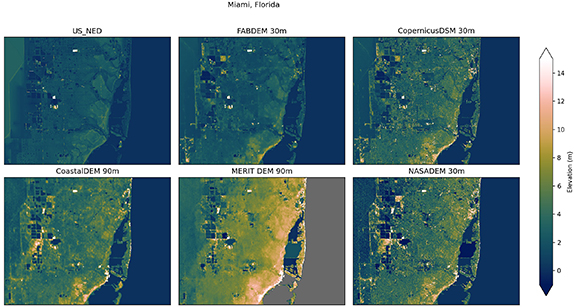
Figure 4. Comparison of different DEMs over a region of Florida, USA including Miami. Domain covers 80.5°–80∘ W, 25.7°–26∘ N. US_NED is the US national elevation data-set (note some of the western extent of this image is not LiDAR).
Download figure:
Standard image High-resolution image
Figure 5. Comparison of different DEMs over a region of the Netherlands. Domain covers 5.268°–5.582∘ E, 51.595°–51.934∘ N. AHN3 is the Netherlands national elevation data-set (as per table S2). Note, some water areas are masked out and shown as grey in the AHN3 panel.
Download figure:
Standard image High-resolution image
Figure 6. Comparison of different DEMs over Fitzroy River, Rockhampton, Australia. Domain covers 150.25°–150.475∘ E, 23.3°  S. LiDAR is referenced in table S2. Note that above 20 m, CoastalDEM does not have corrections applied.
Download figure:
Standard image High-resolution image
Figure 7. Comparison of different DEMs over part of the Mekong delta. Domain covers 106°–106.8∘ E, 10°–10.35∘ N. We did not have access to ground truth LiDAR imagery for comparison at this location.
Download figure:
Standard image High-resolution image
4. Conclusion
This study presents the development of a new global DEM at 30 m grid-spacing, with artifacts from forests and buildings removed (FABDEM). The use of random forest machine learning models is a powerful tool to estimate anomalies in the terrain due to human settlements and forests. The median errors in FABDEM are close to zero and the absolute errors are reduced by up to half in our evaluation against reference DEMs.
Using the gold standard of global terrain data, the Copernicus GLO-30 DEM, gives this data-set an advantage over currently available global DEMs, many of which are derived from the 2000s era SRTM data-set. In comparison to other global DEMs, we find that FABDEM has smaller errors, and importantly resolves fine scale floodplain features which are not resolved by the SRTM based DEMs.
The correction procedure applied in the machine learning model relies on there being sufficient information in the predictor variables to characterise the artifacts we are aiming to correct (forests and building heights). In this study we sourced high quality public data-sets available at a global scale. However, these data-sets do have uncertainties and errors. This is evident in the visual evaluation, for example showing some artifacts from buildings which are not completely removed. Inclusion of more accurate predictor variables in the future will allow for improvements to the machine learning corrections in the future. The underlying Copernicus GLO-30 DEM was found to still have some random artifacts and pits, which were mostly removed by our processing but not completely. Seasonal vegetation anomalies are further difficult to predict. The user should note that the correction is applied in built and forested areas only, and should thus be mindful when using the data in areas where errors are more likely to occur, particularly in areas of steep slopes.
In addition to the predictor variables, reference elevations for training data are key to producing accurate predictions in a machine learning model. A model using training data from one region of the world may be prone to over-fitting and can not necessarily be transferred to other regions. Hence for this study, we used a carefully selected set of reference DEMs from 12 countries around the world to increase the applicability of our models.
FABDEM has notable benefits compared to existing global DEMs, resulting from the use of the new Copernicus GLO-30 DEM and a machine learning correction of forests and buildings. This makes it preferable for many purposes where a bare-earth representation of terrain is needed, such as in hydrology and flood inundation modelling.
Data availability statement
The data that support the findings of this study are freely available for non-commercial use, at the following URL/DOI: https://doi.org/10.5523/bris.25wfy0f9ukoge2gs7a5mqpq2j7.
Acknowledgments
L H and J N were funded by a joint Natural Environment Research Council (NERC) and Vietnam National Foundation for Science and Technology Development (NAFOSTED) project under Grant No. NE/S3003061/1.
We acknowledge the developers of the produces contributing towards this data-set. Specifically, the Copernicus GLO-30 DEM developers, providers of the predictor data-sets (listed in supplementary table S1) and the reference LiDAR datasets (listed in supplementary table S2). We also acknowledge data.bris for hosting the FABDEM data-set.