

Abstract
The worldwide lockdown in response to the COVID-19 pandemic in year 2020 led to an economic slowdown and a large reduction in fossil fuel CO2 emissions (Le Quéré 2020 Nat. Clim. Change 10 647–53, Liu 2020 Nat. Commun. 11); however, it is unclear how much it would slow the increasing trend of atmospheric CO2 concentration, the main driver of climate change, and whether this impact can be observed considering the large biosphere and weather variabilities. We used a state-of-the-art atmospheric transport model to simulate CO2, and the model was driven by a new daily fossil fuel emissions dataset and hourly biospheric fluxes from a carbon cycle model forced with observed climate variability. Our results show a 0.21 ppm decrease in the atmospheric column CO2 anomaly in the Northern Hemisphere latitude band 0–45° N in March 2020, and an average of 0.14 ppm for the period of February–April 2020, which is the largest decrease in the last 10 years. A similar decrease was observed by the carbon observing satellite GOSAT (Yokota et al 2009 Sola 5 160–3). Using model sensitivity experiments, we further found that the COVID and weather variability are the major contributors to this CO2 drawdown, and the biosphere showed a small positive anomaly. Measurements at marine boundary layer stations, such as Hawaii, exhibit 1–2 ppm anomalies, mostly due to weather and the biosphere. At the city scale, the on-road CO2 enhancement measured in Beijing shows a reduction by 20–30 ppm, which is consistent with the drastically reduced traffic during the COVID lockdown. A stepwise drop of 20 ppm during the city-wide lockdown was observed in the city of Chengdu. The ability of our current carbon monitoring systems in detecting the small and short-lasting COVID signals at different policy relevant scales (country and city) against the background of fossil fuel CO2 accumulated over the last two centuries is encouraging. The COVID-19 pandemic is an unintended experiment. Its impact suggests that to keep atmospheric CO2 at a climate-safe level will require sustained effort of similar magnitude and improved accuracy, as well as expanded spatiotemporal coverage of our monitoring systems.
Export citation and abstract BibTeX RIS
1. Introduction
The unprecedented worldwide lockdown in the first few months of year 2020 led to widespread reduced economic activities. As a result, fossil fuel CO2 emissions were reduced by 8% in the first 4 months of 2020 [1] due to reduced transportation, industrial and power generation and an anticipated annual reduction of 4%–7% in CO2 emissions [2]; however, the COVID-19 induced reduction was short-lived as economic activities rebounded subsequently. While the lockdown increased activities such as tele-collaborations that benefit climate, other measures do not lead to the transformation needed in energy systems. Monitoring and understanding such processes from global to local policy-relevant scales are of critical importance for achieving our climate goals. Over the last few decades, the scientific community has been developing worldwide carbon information systems with the aim of monitoring and verification of emissions reduction goals [3–6].
1.1. How big is the impact of this reduction in fossil fuel emissions on atmospheric CO2?
A back-of-the-envelope calculation goes as following. The current fossil fuel emissions rate is 10 GtC y−1 (Gigatonne carbon per year), of which approximately half is taken up by carbon sinks on land and in the ocean, with the remaining half left in the atmosphere, resulting in a CO2 increase of 2.5 ppm per year, as observed in a worldwide network of CO2 observatories such as the renowned Mauna Loa station in Hawaii [7]. Assuming a 7% reduction or 0.7 GtC for the whole year of 2020 (high estimate of [2]), it would cause a 0.18 ppm less increase in global atmospheric CO2 at the end of year 2020 relative to 'business-as-usual' as of 2019.
In reality, the emissions reduction did not occur synchronously in different regions, for example, China in February and Europe, the US and India in March–April (figure S1 available online at stacks.iop.org/ERL/17/015003/mmedia). The estimated reduction of 8% in January–April 2020 [1] corresponds to a decrease of 0.26 GtC, a rather small quantity for atmospheric CO2. However, we expect the COVID signal to largely stay in the Northern Hemisphere (NH) for these few months because atmosphere inter-hemispheric transport takes approximately 1 year. We further assume that the carbon sinks have not started because of dormant winter vegetation and sluggish ocean-atmosphere gas exchange. We therefore expect a 0.25 ppm less increase of NH CO2 at the end of April, assuming that: (a) 2.16 GtC emissions equal to 1 ppm increase in atmospheric CO2; (b) the reduced emissions was majorly located at the NH; (c) and thus COVID anomaly is limited to the NH within the timescale of a few months (e.g. Spring 2020). This magnitude of change is within the capability of today's high-accuracy CO2 analyzers, but small for carbon satellites such as NASA's OCO-2 and the Japanese GOSAT with targeted precisions of ∼1 ppm and their ground calibrations of 0.4 ppm [8–10].
Challenges also arise from the fact that besides fossil fuel emissions, atmospheric CO2 is also strongly influenced by the changes in the biosphere and atmospheric transport in association with weather variability. The growth and decay of the northern vegetation causes a seasonal CO2 amplitude of 6 ppm, while interannual climate variability, such as the El Niño Southern Oscillation (ENSO), causes biogenic CO2 changes of 1–3 ppm [11–14]. Thus, a key question is whether a 0.25 ppm COVID signal can be seen among other (natural) variabilities. The purpose of this study is to investigate the atmospheric CO2 signals resulting from COVID-19 among other natural signals. We explored this question with carbon cycle models and a suite of space-borne and ground-based observations.
2. Results
2.1. To model the atmospheric CO2 response to emissions reduction and biospheric anomalies
We first created a high spatial-temporal resolution fossil fuel emissions ( ) dataset with daily emissions data from a near real time (NRT) product (updated from Liu et al [1]; see section 4). The daily country-level data were disaggregated to model grid resolution based on the Open source Data Inventory of Anthropogenic CO2 (ODIAC) emissions database [15]. As seen in figure 1(a) (detailed temporal evolution in supplementary information figures S1–S2), the carbon emissions intensity decreased by more than 5 gC m−2 mo−1 during February–April 2020 in East Asia, Europe, the US and India, relative to the same period in 2019. While consistent with the temporal variations in the original country-level data [1], the spatially disaggregated data show further emissions reductions concentrated in industrialized regions and areas with high population densities, such as the North China Plain, India's Ganges Basin, and the US Northeast and Midwest, as well as isolated centers such as Sao Paolo.
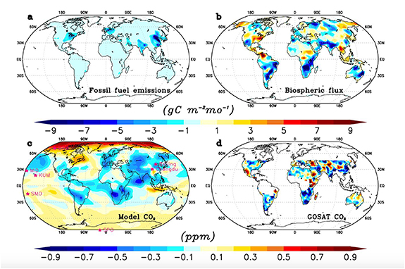
Figure 1. Anomalies for the period of February–April 2020: (a) fossil fuel emissions ( ); (b) terrestrial biosphere-atmosphere flux (FTA); (c) atmosphere transport model simulated column CO2 (vertically averaged); and (d) observed column CO2 from GOSAT. Anomalies in (a) are relative to 2019 while those in (b)–(d) are relative to the climatology of 2010–2019. Fluxes are in gC m−2 mo−1, and CO2 is in ppm. Locations in (c) are selected ground CO2 observation stations for model-data comparison.
Download figure:
Standard image High-resolution imageFor terrestrial biosphere-atmosphere flux ( ), we used a dynamic vegetation and terrestrial carbon cycle model VEGAS [11, 16], while ocean-atmospheric flux came from a multi-model product (see section 4). The biospheric fluxes (figure 1(b)) have regional variations with magnitude often larger than the
  reduction, driven by climate variability. Overall, the terrestrial biosphere had widespread negative anomalies that were particularly strong in the Southern Hemisphere and in April, largely in response to a strong Indian Ocean Dipole event in the circum-Indian Ocean regions [17] (figure S3). As a result, the spatial pattern of net flux
  was dominated by biospheric fluxes.
Because the COVID signal is expected to be confined in the NH (figure S4), we focus our CO2 analysis on the NH region from the equator to 45° N (hereafter NH45). Although the biospheric fluxes dominated both spatial and temporal variability (figure 2(a)), which can be seen that FTA is highly consistent with the Fnet
variabilities, and when summed up over NH45, the magnitude of the 2020  anomaly is larger than that of
  (figure 2(a)). This is because fossil fuel emissions were reduced almost everywhere during the COVID-19 lockdown, whereas the positive and negative anomalies in
  tend to cancel each other out. Consequently, the total flux anomaly Fnet reached nearly −200 MtC mo−1 in April 2020.

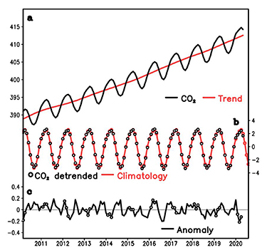
Figure 2. (a) Anomalies of NH fossil fuel emissions ( ), terrestrial biosphere-atmosphere flux (FTA), and net fluxes (Fnet) relative to a 10 year climatology; (b) detrended anomalies of model simulated column CO2, with closed black circles marking each year's February, March and April, while red line is the same but for GOSAT satellite column CO2 data, both averaged for land area between 0° and 45° N (NH45) to make them as comparable as possible. Vertical shading of February–May 2020 indicates the 'COVID-19 period'.
Download figure:
Standard image High-resolution imageSubsequently, these fluxes were used as boundary conditions for the community GEOS-Chem atmospheric transport model for the period of January 2008–May 2020 (see section 4). The output of the model is a four-dimensional depiction of spatial-temporal evolution of atmospheric CO2 that can be compared to various types of CO2 observations, as well as the expected COVID impact (figures S4–S7). Using a method termed DCA (Detrending, Climatology and Anomaly; see section 4), in which a CO2 time series is detrended to remove the low-frequency signal and de-seasonalized to remove the climatological seasonal cycle, we calculated sub-annual anomalies of column CO2, as shown in figure 2(b). After a positive anomaly in January 2020, the CO2 anomaly trended downward, and was 0.21 ppm lower than the long-term climatology in March 2020, and 0.14 ppm lower on average during February–April (figure 2(b) shaded period). This anomaly is the largest for the same season while March 2020 is the lowest month in the last 10 years.
2.2. The GOSAT carbon satellite
Launched in 2009, has collected column CO2 (XCO2) data for over 10 years. The spatial pattern of February–April 2020 GOSAT anomalies (figure 1(d)) is similar to the model over India, southern Africa, South America and the central US where large negative values are wide-spread, although the overall spatial correlation is weak (figures 1(c) and (d)). Detailed monthly evolution shows similar broad patterns of agreement, as well as larger detailed differences (figures S8 vs. S9). The time series of CO2 anomalies averaged over NH45 (figure 2(b)) shows reasonable agreement, mostly within GOSAT's uncertainty range (see section 4 and figure S10), with a correlation coefficient of 0.43. The differences may originate from two main sources: (a) the satellite's sparse spatial-temporal sampling, particularly at higher latitudes and cloudy regions; and (b) errors in atmospheric transport model and simulated biospheric fluxes. The drop during February–April 2020 discussed above is also clear in GOSAT, although the signal is at the border of being statistically significant (figure 3(d)).
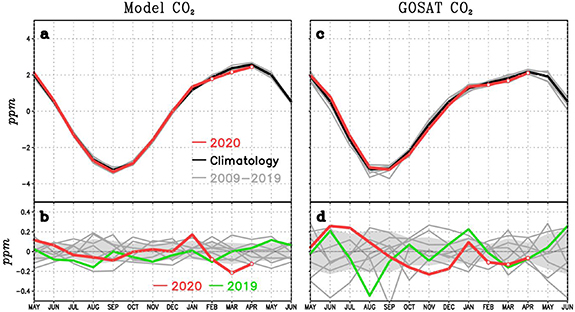
Figure 3. (a) Seasonal cycles of detrended modeled column CO2 averaged over 0–45° N (NH45) land region, with each individual year plotted in gray lines, climatological mean of the 10 years of 2009–2019 in black, and most recent year May 2019–April 2020 in red; (b) CO2 anomalies relative to the climatology in (a) with same color scheme, and green for the previous year (May 2018–April 2019); (c)–(d) As in (a)–(b) but for the GOSAT satellite observed column CO2.
Download figure:
Standard image High-resolution imageTo better appreciate how unusual year 2020 was, we plotted the CO2 seasonal cycle from May 2019 to April 2020 (called Year 2020) against those of the previous 10 years (figure 3). The CO2 anomaly for the model is outside the standard deviation of the previous 10 individual years, while it is just at the border of being statistically significant for GOSAT, which has almost twice as high a variance; this finding is not surprising given its sparse spatial-temporal coverage. Even though the COVID signal is small, the model-data consistency in the above analysis supports using both model and satellite column CO2 for short-term anomaly detection.
In addition to the NH, we also conducted similar analyses at global and regional scales of interest. For the larger region of 45° S–45° N (G4545), both the model and GOSAT show somewhat clearer negative anomalies in 2020 (figures S11 and S12). The more robust 45° S–45° N signal captures the spatially more coherent biospheric anomalies in the Southern Hemisphere. In the other direction at the regional scale, a large decrease in Eastern China in February 2020 is seen (figure S13), which is consistent with the expectation of the large emissions reduction from China during the COVID lockdown. However, it is not statistically significant, and the spatial and temporal patterns are not consistent between the model and the observation.
2.3. To attribute the 2020 CO2 drawdown to the biosphere, atmospheric transport (weather), and COVID-caused reduction in fossil fuel emissions
We conducted two additional model sensitivity experiments to delineate these effects (see section 4). The monthly evolution of CO2 anomalies from these experiments (figure 4) indicates that the roles of the biosphere, weather, and COVID vary from month to month. In February–April 2020, the biosphere in NH45 had positive but decreasing anomalies while the COVID effect steadily increased. The weather effect was large in February and March to drawdown CO2, but small in April (all in comparison with 2019 by model design). Averaged over February–April, the biosphere contributed 0.042, weather contributed −0.086, and COVID contributed −0.096 ppm, leading to an average of −0.14 ppm CO2 change (drawdown) while March alone was −0.21 ppm.

Figure 4. Model sensitivity experiments to separate the effects from the three factors: biospheric flux (B), atmosphere transport (weather or W), and COVID-19 induced reduction in fossil fuel emissions (C). Starting from the original experiment that has all three effects of biosphere, weather and COVID (BWC), experiment BW removes the COVID impact, while experiment B removes both the COVID and weather impacts. By experimental design, the biospheric effect is relative to a 10 year climatology while COVID and weather effects are relative to 2019 (see section 4). Cumulative contribution to mean column CO2 anomalies over 0–45° N are shown (NH45). The difference of two experiments represents the contribution from an individual factor.
Download figure:
Standard image High-resolution imageIn summary, the three factors impacted CO2 in intricate ways. In the period of February–April 2020, while the biosphere of the Southern Hemisphere had widespread CO2 uptake, the NH had some uptake in South Asia and Siberia that was overridden by CO2 release from other regions, partially in response to a warm winter (figure S3). In contrast, COVID emissions reduction was the most spatiotemporally consistent factor in the NH, contributing to majority of the CO2 decrease. The weather impact on CO2 fluctuated from month to month but contributed a significant portion of the CO2 drawdown in the NH during February–March 2020. Its importance rises towards smaller scales to which we turn our attention now.
2.4. We analyzed data from atmospheric background CO2 stations
From the GLOBALVIEWplus dataset ObsPack [18] (see section 4). Figure 5 compares the model with surface observations at five marine boundary layer stations that span the remote Pacific region from north to south. Flask sampling at these sites is carefully conducted to represent atmospheric background concentrations on the scale of hundreds to thousands of kilometers.

Figure 5. Model-data comparison of sub-annual CO2 anomalies (ppm) at five atmospheric background sites: Barrow, Alaska (BRW); Midway Island, North Pacific Ocean (MID); Cape Kumukahi, Hawaii (KUM); American Samoa in South Pacific Ocean (SMO), South Pole Station. Site locations are marked in figure 1(c). Similar to figure 2(b), the model is in black, and the observation is in red, with filled markers indicating the months of February–April for each year. Data are shown only for the recent few years, while anomalies are relative to a 10 year climatology. The model-data correlation coefficients for the five stations are 0.53, 0.45, 0.55, 0.30, −0.02 respectively. Shading indicates uncertainty (section 4).
Download figure:
Standard image High-resolution imageThe anomalies at Kumukahi (KUM) are relatively small in February and March 2020, but decrease rapidly to lower than −1 ppm in April. The model and observations are broadly similar, in particular, the decrease in April. It is tempting to associate this drop with COVID reduction. However, a closer look at the model sensitivity experiments (figure S14) reveals large month-to-month fluctuations from the biosphere and weather, for example, a positive anomaly up to +1 ppm from the biosphere and a similarly large negative anomaly from weather in March. Of the total CO2 drop by 1 ppm in April, 0.5 comes from the biosphere, 0.5 from the weather, and only 0.2 ppm from COVID.
Unlike a decrease in Hawaii, CO2 at Barrow, Alaska (BRW) shows an increase in early 2020, while Midway Island in the North Pacific Ocean (MID) has a decrease in February–March and rebounds in April, both of which are attributable to the biosphere and/or weather (figure S14). Thus, while the sub-annual signal of 1–2 ppm at these marine surface stations is a few times larger than the global mean column anomalies seen by the satellite, the variability at a given station is dominated by the biosphere and weather. Nevertheless, the 0.1 ∼ 0.2 ppm decrease due to COVID-19, although smaller than the biospheric and weather effects, is separable using the model, and is consistent with the global-scale COVID induced drop discussed above. The overall consistency between the model and station observations suggests the ability of both the model and observation in capturing these sub-annual changes, regardless of the origin.
2.5. City-scale CO2 changes
Because a major fraction of emissions comes from cities with high levels of human activities, one can expect a large COVID signal in urban CO2 data. We analyzed CO2 measurements in Beijing and Chengdu.
Surface observations in Beijing show CO2 for the winter-spring (December 2019–April 2020) compared with the same period the year before (figure 6(a)). During the pre-COVID period of December–January, CO2 was significantly higher in 2020 than in the year before, because this winter's atmosphere was more stable and less 'ventilated'. February was dominated by two high-CO2 weather events, one in each year. We compared the wind speed of 2020 winter with 2019 based on the 0.25° × 0.3125° high resolution GEOS-FP modeling dataset. And the data showed that the mean daily wind speed is indeed much smaller around 1 February (1–3 m s−1 in 2020 compared with those 3–8 m s−1 in 2019), which contributed to the higher enhancement in 2020. The expected low CO2 values due to COVID in January–February (figure 6(b)), as 'predicted' by the model, do not have a clear correspondence in the weather-dominated CO2 observations. In general, the modeled magnitude of change is much smaller than the variability. During March–April, the difference between the 2 years decreases to much smaller values. We computed the enhancement for the shading period, and it is 30 ppm in 2020, compared with the 20 ppm in 2019. It is tempting to explain this difference as the result of emissions reduction, but it is mostly brought about by weather regime shifts in the spring season with dominantly northwesterly wind from the Mongolian Plateau. Thus, although the COVID-19 signal is large, it is 'buried' in even larger weather noise. Other cities are similarly dominated by weather, for example, a monthly drop of 1–2 ppm in New York City and Delhi, and an increase of 1–2 ppm in Washington DC and Paris (figure S15).

Figure 6. Daily CO2 mole fraction measured in Beijing. (a) Measured CO2 enhancement (Xianghe station (a near-city site) minus Xinglong, a rural site in the mountains northeast of Beijing, for the period of November 2019–April 2020 (labeled as 2020)), compared with the year before (November 2018–April 2019, labeled as 2019); (b) model simulated CO2 difference caused by COVID-19 emissions reduction (experiment BWC—experiment BW). Vertical shading indicates the lockdown period in Beijing.
Download figure:
Standard image High-resolution imageInterestingly, CO2 measured in the city of Chengdu shows a stepwise drop on January 24, the day before the traditional Chinese Lunar New Year, followed by a city-wide lockdown with little urban activity for the next 1–2 months (figure 7). The difference between the month before and after the lockdown is more than 20 ppm, and the abrupt change on the time scale of one day is consistent with a COVID signal, and there is no other known mechanism to explain this result. Concurrent particulate matter (PM2.5) measurements support this interpretation because the short-lived PM2.5 has a similar pattern on timescales shorter than a few days, but it has much less monthly and longer timescale variations compared to CO2.

Figure 7. Hourly CO2 and PM2.5 measured in Chengdu, a city in the Sichuan Basin to the east of Tibetan plateau. An abrupt drop on 24 January 2020, following the Lunar New Year and city-wide lockdown is clearly visible.
Download figure:
Standard image High-resolution imageWhy is the COVID signal clear in Chengdu, but not in Beijing? The answer lies in the differences in weather. Chengdu, which is situated within the Sichuan Basin in southwestern China, is surrounded by great mountain ranges including the Tibetan Plateau and has generally very calm weather with a famously known atmospheric inversion layer that is rarely broken [19], whereas Beijing, which is at the edge of the North China Plain, is subject to large weather fluctuations, frontal passages and seasonal shifts. Thus, weather variation is relatively small in Chengdu to allow COVID signal to be revealed. And the simulations in Chengdu also confirmed a 1–10 ppm reduction resulted from COVID-19 during the lock-down period (compared with the observed 30 ppm), despite of the coarse resolution and fossil fuel emissions data. And the smaller modeled signal can be attributed to two potential reasons: (a) Lacked of local emissions reductions data for model input, which is substituted by national average value of −18.4% in February, and this was likely to be underestimated through communications with local inhabitants; (b) The spatial mismatch. Considering the instrument is deployed on the rooftop of a 6th floor building that is near a traffic line, and thus the observed signal reflected more of the traffic emissions reductions.
2.6. Direct observations of on-road CO2 concentrations
Have been conducted in Beijing periodically since 2017 using mobile platforms [20, 21] (see section 4). Some of these 'CO2-tracking' trips took advantage of light-weight low-cost CO2 sensors [22]. Three trips were selected from before, during, and after the COVID-19 lockdown while minimizing differences in other factors such as weather conditions, rush hours, and weekend effects. The average CO2 is 513 ppm before, 455 ppm during, and 501 ppm after the height of lockdown (figure 8). To further remove the confounding effect of still somewhat different weather conditions, we subtracted the CO2 concentration measured at the Institute of Atmospheric Physics (IAP) tower station. This difference can be thought as a traffic-induced on-road 'CO2 enhancement' relative to a 'city background'. This 'traffic enhancement' is 65, 30 and 50 ppm respectively for the three periods. The more than 30 ppm less traffic CO2 during COVID, and still somewhat low value during recovery, is consistent with direct traffic data, which is not surprising, because the reduced transportation is the largest contributor of CO2 reduction during lockdowns in cities.
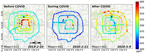
Figure 8. On-road CO2 concentrations measured before, during and after the COVID-19 lockdown in Beijing. These 'CO2 tracking' car trips covered the city's four major transportation arteries, from the Second (innermost) to the Fifth Ring Road. The west-east distance of the Fifth Ring Road is about 30 km. Each dot is 1 min average of the original 1 s or 2 s data. Station data from the IAP tower, marked by black triangle, was used as 'city background' to compute on-road enhancement.
Download figure:
Standard image High-resolution image3. Discussion
The detectability of the COVID-19 CO2 signal depends strongly on spatial and temporal scales. Our results show that, consistent with model prediction, the GOSAT carbon satellite is able to detect a short-term global mean CO2 anomaly decrease of approximately 0.2 ppm in the NH, a number below the satellite instrument's targeted accuracy of individual measurements. This somewhat surprising result stems from the fact that the COVID reduction is negative nearly everywhere while the biosphere signal varies strongly spatially. Over large regions such as NH45, the spatial averaging compensates for satellite sampling sparsity, while the biosphere and weather effects tend to cancel each other out. As a result, the drop in global-scale CO2 anomalies was dominated by the spatially coherent COVID signal. One implication for detection is the need for meticulous approaches in enhancing signal-to-noise ratio and maximizing spatial-temporal data coverage [23, 24]. Here, a critical perspective is the focus on sub-annual time scales, which have received little attention in the past compared with the much larger CO2 seasonal cycle and interannual variability. Our results suggest that current observation and modeling capabilities can depict sub-annual variations with some consistency, and according to the model, the COVID period had the largest sub-annual CO2 anomaly in the last 10 years. We also note that what we call 'COVID-induced reduction' here is relative to the 2019 emissions level. In a business-as-usual scenario, emissions are likely to increase which may lead to a larger 'anomalous reductions'.
The anomalies in surface observations of the atmospheric background CO2 concentration have sub-annual signals of 1–2 ppm, which is substantially larger than the ∼0.2 ppm COVID fossil signal. However, the modeling results are sufficiently realistic in capturing sub-annual variabilities consistent with station observations, lending support in using model experiments to separate the COVID effect from the larger weather and biospheric variability.
At the urban scale in many cities such as Beijing, New York City and Paris, atmospheric variability dominates. Seasonal variations in weather patterns prevented us from confidently discerning the COVID signal despite the large fossil fuel emissions changes expected there. Of course, this does not exclude in any way the possibility of atmospheric inversion systems to find the fossil fuel signal by using atmospheric transport to solve for flux directly, as has shown by Weir et al [25]. A major caveat is that the model resolution is too coarse to resolve the cities properly and the real signal is likely stronger than seen here and it would be better simulated by meso-scale models. Moreover, where weather variability is modest, such as in Chengdu, the lockdown caused a clear CO2 drop. Additionally, decrease in on-road CO2 enhancement larger than 20 ppm in Beijing was observed, which is perhaps the most direct observation of a localized emissions reduction.
Despite the dramatic reduction in economic activities during the 2020 COVID-19 worldwide lockdown, the short-duration of the event has left only a small signature in the atmospheric CO2 which results from fossil fuel emissions accumulated over two hundred years due to CO2's long atmospheric life-time. Nevertheless, our analysis demonstrates that its global-to-local impacts are already detectable from a wide variety of observation platforms we have (e.g. ground, aircraft and satellites), albeit still imprecise, by current carbon monitoring systems using a variety of approaches, and that meaningful causality attributions to fossil fuels, the biosphere and weather can be made by combining the model and observations. Continued improvement and expansion of such capabilities can play a critical role in monitoring and verification of fossil fuel emissions reduction targets at policy-relevant scales, such as local, country, and global scales [26]. They can also facilitate climate mitigation efforts from governments, cities, institutions and citizens.
4. Materials and methods
4.1. Atmospheric transport model simulation
To simulate the atmospheric CO2, the model solves the carbon mass balance equation as follows:
where  is the atmospheric CO2 growth rate,
  is fossil fuel emissions,
  is terrestrial to atmosphere flux,
  is ocean to atmosphere flux, and
  is net surface to atmosphere flux. The model is run in a 'forward' fashion for each three-dimensional model grid point (location), forced by the three fluxes, as well as meteorological variables for atmospheric transport and mixing. Here we use the GEOS-Chem atmosphere transport model v12.5.0 (http://acmg.seas.harvard.edu/geos/) at a horizontal resolution of 4° × 5° with 47 vertical levels. The fluxes (below) at different resolutions are re-gridded to 4° × 5°. The model is driven by the meteorology field MERRA2 from the NASA Global Modeling and Assimilation Office. Details of the setup and evaluation were described previously [27, 28]. The simulation period was from 1 January 2008 to 31 May 2020, and data after January 2010 were used for analysis.
4.2. Fossil fuel CO2 emissions
 combines a number of sources, including the Global Carbon Project (GCP) annual country-level carbon budget for 1959–2018 [29] with updates for 2019 by Le Quere et al [2], daily data for 2019–2020 from Liu et al [1], the TIMES hourly scaling factor of Nassar et al [30], and the spatial information of the ODIAC database of Oda et al [15].
Recently, a daily resolution, country-level data became available [1]. This novel dataset achieved daily resolution by taking advantage of a variety of sector-based energy and economic activity statistics, including real-time traffic data and daily electricity generation data of major power suppliers. However, the Liu et al [1] data were available only for early 2019 and 2020, and for this work, it was updated to cover the period of January 2019 through May 2020. For the years 2008–2018 when we do not have daily resolution data, we use the 2019's daily variation as a surrogate but retain their annual total. Because the emissions of Liu et al [1] for 2019–2020 are slightly different from GCP, in order to maintain the consistency of  from 2018 to 2019–2020, we use the country-level GCP fossil fuel values as a constraint to rescale the yearly total
  from 2008 to 2020, and the same scaling factor for 2019 is used for 2020 to obtain a harmonized time series. Furthermore, we combine the diurnal scaling factor from the TIMES method of Nassar et al [30] and the daily national CO2 emissions of 2019 of Liu et al [1] to obtain hourly country-level CO2 emissions in 2019 and 2020.
The gridded spatial information comes from the ODIAC emissions [15]. ODIAC uses the annual country-level fuel consumption based on CO2 emissions estimates [31] and disaggregates to a 1 km or 1 degree resolution using satellite night light observations and point source data. The annual data were disaggregated to monthly based on a climatological seasonal cycle. Here we simply disaggregated the country-level hourly data above to 1° × 1° with the spatial information of ODIAC. Since COVID-19 reductions are more concentrated in cities with a major reduction in transportation [1, 32], this disaggregation in proportion to ODIAC's spatial pattern may underestimate the reduction in metropolitan regions.
Altogether, the method can be summarized in the following equation for 2008 ∼ 2018:
and for 2019 ∼ 2020:
where y is the year, th is the hour, td is the day, tdiurnal is the diurnal cycle. c is country, i is longitude, j is latitude, and tot is the yearly total value.  is the emission of country c at location i, j at time th of the year i. The four datasets used to obtain this harmonized labeled ODIAC, GCP, TIMES and LZ, where LZ is the updated Liu et al [1] dataset.
4.3. The terrestrial biospheric flux
 is simulated by a dynamic vegetation and terrestrial carbon cycle model VEGAS [11, 16]. The model is forced by observed climate variables including monthly precipitation, hourly temperature and radiation, and historical land use patterns, as well as atmospheric CO2. The model was run at hourly time step and 0.5° × 0.5° resolution from 1901 to April 2020. This version 2.6 of VEGA largely S follows the simulation protocol of the TRENDY [33] and the MsTMIP [34] terrestrial model intercomparison projects with some model and NRT forcing data updates. Carbon cycle models have been extensively applied to long-term, interannual and seasonal variations, but rarely in sub-annual changes of interest here. VEGAS has been shown to be among the models better at simulating such short-term changes [35, 36].
4.4. The ocean-atmosphere carbon flux
 uses the spatial pattern of pCO2 observation derived fluxes from Takahashi et al [37]. To obtain the temporal variation, we rescaled the Takahashi spatial pattern for the year 2013 with the temporal evolution of
  from the GCP annual carbon budget analysis which is based on estimates from multiple ocean carbon cycle models [29]. The carbon budget was only available up to 2018. For the year of 2019 and 2020, the GCP ocean values were linearly extrapolated using the values from the previous 10 years. The annual carbon budget thus does not contain a possible sub-annual contribution from the ocean, which is generally believed to be small compared with land and fossil flux anomalies.
4.5. Model sensitivity experiments
To delineate the contribution to CO2 changes from fossil fuel emissions  , biospheric flux
  , and weather, we designed three sets of experiments:
- (a)BWC (biosphere + weather + COVID): the full experiment described above with realistically varying biospheric fluxes
 , weather, and including COVID-induced emissions reduction.
 - (b)BW (biosphere + weather, no COVID): same as in BWC, but replacing of 2020 with that of 2019.
- (c)B (biosphere only): same as in BW, but replacing all years' meteorology values (wind, etc) with that of 2019.


Thus, compared with BWC, experiment BW removes the effect of COVID emissions, while Experiment B further removes the weather effect. The differences among these experiments show the effect on CO2 of each individual factor. In figure 4, the anomaly for experiment B is calculated as a detrended anomaly, while those of BW and BWC represent the differences between 2020 and 2019, following the experimental design.
4.6. Observations and analysis of column CO2 from the GOSAT satellite
The satellite column CO2 data are Level-3 products from the National Institute for Environmental Studies (NIES) [24] (www.gosat.nies.go.jp/en/about_5_products.html). The L3 data were derived from the L2 data with spatial interpolation using the Kriging technique. The data is at 2.5o × 2.5o resolution and available from August 2009 to April 2020, and these data were gap-filled with the spline method. There are known biases in oceanic glint data, so we only used land data in our analysis. For this reason, regional average analyses in such as figure 2(b) are over land only for both the model and GOSAT to facilitate comparison. Additional uncertainty comes from missing GOSAT data in regions such as the core of the Amazon due to persistent cloud cover and the northern boundaries where a large solar zenith angle may lead to larger uncertainty (e.g. figure 15 in [24]). Thus, we excluded grid points with data coverage less than 63% and applied a spline fit to fill the gaps for the remaining data.
4.7. Global network of surface CO2 observations
The surface station data are from the GLOBALVIEWplus ObsPack framework [18] that collects a great variety and numbers of in-situ, flask sampling, aircraft and other CO2 measurements. The five stations data used in our analysis are all flask sampling data. These are baseline stations managed by NOAA that have been in operation for several decades. Great care is taken to sample air representative of large-scale atmospheric background conditions. The data product used here is GLOBALVIEWplus 5.0, with the most recent update ObsPack NRT (obspack_co2_1_NRT_v5.2_2020-06-03) provided by NOAA's CarbonTracker team [38, 39]. The most recent year's data have been quality-controlled by an automated procedure, and they may still be subject to modifications from further manual quality control.
4.8. Uncertainty estimates of observational data
We evaluated the impact of measurement uncertainty on our results, as shown in figure 2(b) (satellite) and figure 5 (ground stations). For GOSAT, we first took its location-specific measurement uncertainty produced by the GOSAT team (figure S10(a)). We then used a Monte Carlo method to generate an ensemble of spatially correlated uncertainty maps using the statistical method of joint multivariate Gaussian distribution. For each ensemble member, each location (model grid point) was assigned a random error drawn from a Gaussian distribution with the standard deviation from the GOSAT measurement uncertainty map. A spatial correlation scale of 1000 km was assumed in the multivariate covariance matrix. Sensitivity experiments using correlation scale of 2000 and 5000 km showed similar final results. The errors were then added to the CO2 value at the corresponding locations. A total of 100 such maps (realizations) for any given month were generated, with 8 shown in figure S10(b). An uncertainty range was computed for any given regional mean CO2 (figure S10(c) and figure 2 of main text). This task is simpler for a ground station, where we just used the within-month standard deviation as the uncertainty because it does not involve spatial correlation.
4.9. City CO2 station observations
A network of six tower stations using high accuracy Picarro CO2 analyzers has been running since 2018 as part of the Beijing-Tianjin-Hebei (JJJ) carbon monitoring project [21], run by the Chinese Meteorological Administration and the IAP of the Chinese Academy of Sciences. The CO2 analyzers were calibrated four times a day, with calibration gas tracing to the World Meteorological Organization standard. The data have a nominal accuracy of 0.1 ppm. A network of low-cost CO2 sensors has been running in various stages of development since 2016, as a collaborative effort among the IAP, the University of Maryland, and the US National Institute for Standards and Technology. These sensors were found to be able to achieve an accuracy of ∼5 ppm after calibration and environmental correction [22]. The data used in this paper for Beijing stations were measured with Picarros while the data in Chengdu were from a low-cost sensor node with three individual CO2 sensors.
4.10. On-road CO2 observations in Beijing before, during and after the COVID-19 lockdown
We conducted several on-road CO2 measurements in Beijing and the surrounding area using mobile platforms before, during and after the COVID-19 lockdown. Because urban CO2 concentrations are strongly influenced by weather, we selected three trips with the closest weather as possible for the days of 20 February 2019, 21 February 2020, and 9 May 2020. Additionally, we calculated the on-road CO2 enhancement relative to a city 'background' measured at the IAP tower station. We used CO2 sensors of different accuracies, including Picarro and LI-COR LI-7810, both mounted inside a car with an air inlet from above roof [20]. We also used low-cost sensors mounted on windshields, and these sensors were calibrated before and after each trip [21]. Some of the sensors were in the same car as Picarro and their agreement was within 5 ppm. A detailed analysis of these trips and methodology are described in D. Liu et al [40].
4.11. Analysis of CO2: separate sub-annual anomalies from trend and seasonal cycle
Atmospheric CO2 data contain variabilities on a variety of time scales, from long-term increasing trends driven by fossil fuel emissions and carbon sinks [41], decadal variations [42], and interannual variability dominated by ENSO [11], to a prominent seasonal cycle [16, 43] in response to the annual growth and decay of the biosphere. The possible COVID-19 signal of interest here lasts for a few months on sub-annual (month to intra-seasonal) timescales. Monthly-scale high-frequency variabilities are generally less well studied and are often filtered out so as to focus on seasonal and longer-term changes [44].
Here, we calculate sub-annual anomalies using a four-step 'detrended anomaly' approach termed DCA:
- (a)A 12 month running mean is applied to the original CO2 data. The running mean mostly contains signals longer than a year, including long-term trends, and interannual to decadal variations (figure 9(a)).
- (b)This running mean is then subtracted from the original CO2 data. The result is considered 'detrended' and is dominated by seasonal cycles (figure 9(b) black line).
- (c)A climatology is then calculated as the mean seasonal cycle (figure 9(b) red line).
- (d)The sub-annual anomalies (detrended anomalies) are the differences between the detrended CO2 and its climatology.
Figure 9. The DCA method for finding sub-annual anomalies in a typical CO2 time series (model simulated global mean CO2 are shown). (a) Original CO2 data (black) and 12 month running mean (red); (b) CO2 detrended (black) and its climatology (red); (c) detrended anomalies (CO2 detrended minus its climatology), with open circles marking February–April of each year.
Download figure:
Standard image High-resolution image
The approach using running mean or other filtering techniques to obtain low-frequency signals has been widely used to study CO2 variability [16, 33, 44, 45]. The last two steps consist of a standard definition of climatology and anomaly. The final sub-annual signal is thus detrended (low-frequency removed) and de-seasonalized (climatological seasonal cycle removed). In comparison with the DCA method, the standard climatology/anomaly method (simply called the CA method here) does not involve detrending, and it retains a low-frequency signal. Therefore, the DCA method is suitable for finding CO2 sub-annual anomalies, while the CA method is used for flux analysis, such as in figure 2(a), which contains both interannual and sub-seasonal information.
Acknowledgments
We are grateful to the providers of the following datasets, made available in a timely fashion: the GOSAT satellite data by JAXA and NIES, the GLOBALVIEWplus ObsPack data via Andy Jacobson, Kirk Thoning and Pieter Tans, the NASA GISS temperature data and NOAA CPC PREL/OPI data. We thank the students and volunteers involved in the Beijing carbon monitoring project, in particular the CO2-tracking trips. We benefited from discussions with Ruqi Yang, Wenhan Tang, David Crisp and Chris O'Dell on detecting COVID signal, and Anna Karion, James Whetstone, Israel Lopez-Coto on sensor development and regional CO2 modeling. We acknowledge support from MOST (2017YFB0504000), NOAA (NA18OAR4310266), and NIST (70NANB14H333).
Data availability statement
The fossil fuel data are available at carbonmonitor.org. The VEGAS biospheric flux data are available at www2.atmos.umd.edu/~cabo/NRT/. The GOSAT data are available at https://data2.gosat.nies.go.jp/index_en.html. The ObsPack data are available at www.esrl.noaa.gov/gmd/ccgg/obspack/data.php. And the fossil fuel emissions data for model are available at http://iark.cc/∼liuzq/COVID-CO2/ODIAC.nc.
The data generated and/or analysed during the current study are not publicly available for legal/ethical reasons but are available from the corresponding author on reasonable request.
Code availability
The GEOS-Chem model is a community model and the code is available at http://acmg.seas.harvard.edu/geos/.
Author contribution
NZ, PH, DL and RD designed the study. NZ and ZQL designed and ZQL conducted the model simulations. CM, DL, RD, and ZQL did the model development. QC conducted the biosphere model simulations. ZL, TO, ZQL, NZ, PH produced the fossil fuel emissions data. TO and SM provided GOSAT interpretation. PH, BY, PW, WS, NZ, and DL organized the observations and CO2-Tracking trips in Beijing. NZ, ZQL and DL led the analysis and wrote the paper, and all participated in synthesis and helped writing.
Conflict of interest
The authors declare no competing interests.