

Abstract
Quantifying the drivers of terrestrial vegetation dynamics is critical for monitoring ecosystem carbon sequestration and bioenergy production. Large scale vegetation dynamics can be observed using the leaf area index (LAI) derived from satellite data as a measure of 'greenness'. Previous studies have quantified the effects of climate change and carbon dioxide (CO2) fertilization on vegetation greenness. In contrast, the specific roles of land-use-related drivers (LURDs) on vegetation greenness have not been characterized. Here, we combined the Interior-Point Method-optimized ecosystem model and the Bayesian model averaging statistical method to disentangle the roles of LURDs on vegetation greenness in China from 2000 to 2014. Results showed a significant increase in growing season LAI (greening) over 35% of the land area of China, whereas less than 6% of it exhibited a significantly decreasing trend (browning). The overall impact of LURDs on vegetation greenness over the whole country was comparatively low. However, the local effects of LURDs on the greenness trends of some specified areas were considerable due to afforestation and urbanization. Southern Coastal China had the greatest area fractions (35.82% of its corresponding area) of the LURDs effects on greening, following by Southwest China. It was because of these economic regions with great afforestation programs. Afforestation effects could explain 27% of the observed greening trends in the forest area. In contrast, the browning impact caused by urbanization was approximately three times of the greening effects of both climate change and CO2 fertilization on the urban area. And they made the urban area had a 50% decrease in LAI. The effects of residual LURDs only accounted for less than 8% of the corresponding observed greenness changes. Such divergent roles would be valuable for understanding changes in local ecosystem functions and services under global environmental changes.
Export citation and abstract BibTeX RIS

Original content from this work may be used under the terms of the Creative Commons Attribution 4.0 license. Any further distribution of this work must maintain attribution to the author(s) and the title of the work, journal citation and DOI.
1. Introduction
Changes in vegetation growth can affect the surface energy, carbon, and water budgets through a series of biophysical processes thus, have important implications for hydrology, ecosystems, and climate (Forzieri et al 2017, Zeng et al 2017, 2018, Xie et al 2019, Lian et al 2020). At large spatial scales, changes in vegetation are commonly derived from the satellite-observed leaf area index (LAI) or normalized difference vegetation index, providing a measure of changes in biomass and 'greenness' (Mao et al 2016, Zhu et al 2016, Zhang et al 2017, Zhao et al 2018, Piao et al 2020). During recent decades, the widespread greening of the Earth has been documented by satellite observations due to rapid environmental changes (Zhu et al 2017, Tharammal et al 2018, Chen et al 2019b, Myers-Smith et al 2020, Peng et al 2020, Piao et al 2020). As a result, quantifying the drivers of vegetation greenness has become a hot topic in global change research to understand the changing mechanisms of terrestrial ecosystem functions and services.
Several recent studies investigated the drivers of vegetation greenness across multiple scales (Lu et al 2016, Mao et al 2016, Kong et al 2017, Li et al 2017, Wang et al 2018a, 2018b, Emmett et al 2019, Berner et al 2020, Liu et al 2020, Xu et al 2020). Drivers of vegetation greenness in terrestrial ecosystems can generally be attributed to multiple interacting biogeochemical factors and land-use-related drivers (LURDs) (Zhu et al 2016, Mendoza-Ponce et al 2018, Chen et al 2019b). Biogeochemical factors include changes in the atmospheric carbon dioxide (CO2) concentration, changes in meteorological factors (such as temperature and precipitation), and the deposition of nitrogen. Besides, these factors also interact with LURDs. Note that LURDs have been described as land-use effects or land-change processes in previous studies (Tharammal et al 2018, Yin et al 2018, Wang et al 2018a). The LURDs include land cover change, human land-use management, and natural disturbances, involving agricultural advancement, afforestation, overgrazing, urbanization, biodisasters, and fire disasters (Malhi et al 2008, Liu et al 2016, Song et al 2018). Previous studies have generally quantified the effects of biogeochemical factors and land cover change on vegetation greenness at global scales, as well as the importance of local effects of LURDs on observed greenness change (Mao et al 2016, Zhu et al 2016, 2017, Li et al 2017, Chen et al 2019a). Moreover, the dominance of the different LURDs shows a strong spatial variation between regions (Zhu et al 2016, 2017, Song et al 2018, Wang et al 2018a). Several earlier studies have investigated the effects of single to three LURDs on vegetation greenness using statistical analyses at a regional level, especially across China (Piao et al 2015, Hua et al 2017, Li et al 2017, Wang et al 2018a, Wu et al 2019). However, the roles of a few LURDs on changes in vegetation greenness have been emphasized rather than fully quantified in these previous studies. China has experienced drastic land use change with noticeable vegetation dynamics due to its rapid socio-economic development and the implementation of several land management policies since the beginning of the 21st century (Liu et al 2010, 2014, Piao et al 2015, Chen et al 2019b). Various LURDs play different roles in vegetation greenness across China (Li et al 2017, Qu et al 2018, Wu et al 2019, Gao et al 2020). For example, urbanization due to population growth contrasts with afforestation programs. The negative effects of urbanization and the positive effects of afforestation could be superimposed and complicated. Therefore, it is necessary to disentangle the roles of various LURDs on vegetation greenness in China.
Two sorts of techniques have been primarily implemented to estimate the contribution of driving factors to vegetation greenness. The first one is based on statistical approaches such as correlation or regression analysis (Los 2013, Lü et al 2015, Wu et al 2015, Xiao et al 2015, Hua et al 2017, Jiang et al 2017, Qiao et al 2020). The statistical approaches are simple but suffering from potential limitations in explaining the attribution of the greenness change (Piao et al 2015, Zhu et al 2017). It can explain that there is a correlation between two variables, but it does not mean causality. They generally evaluate the effects of environmental variables on vegetation growth by assuming a linear relationship between the vegetation growth and its environment rather than assuming a non-linear relation between them. They even cannot distinguish the attribution of the annual fluctuation and trends in vegetation growth.
The second technique is using process-based ecosystem models driven by observed environmental variables. The net contributions of environmental factors to vegetation greenness could be determined by the factorial simulation, which is the difference between the results in the scenarios considering a specified factor or not (Piao et al 2006, Zhu et al 2017). This ability to effectively separate the contributions of different driving factors to vegetation greenness is the great advantage of using the ecosystem process models (Piao et al 2020).
However, the ecosystem model-based method does have some limitations as well. First, there are significant uncertainties when the single ecosystem model is used for vegetation simulation because it is region-specific in model structure, driving parameters, and performances of different ecosystem models (Zhu et al 2016, 2017). Previous studies have generally used several optimal strategies, such as the multimodal ensemble mean method, to optimize the integration of ecosystem model simulations to reduce the uncertainty of a single ecosystem model simulation (Zhu et al 2016, 2017). Moreover, Tang et al (2021) recently demonstrated that the interior-point method (IPM) performance for optimizing the integration of the multi-ecosystem model ensemble is better than that of the other methods that have often been used in previous studies. Thus, the IPM was induced to optimize the integration of multi-ecosystem model simulations in this study.
Second, given the lack of the isolated scenario simulations related to detailed land-change processes, there may be uncertainty in the roles of various LURDs on vegetation greenness quantified by the ecosystem model-based method (Le Quéré et al 2015, 2016). To make up this limitation of the ecosystem model-based method, the specific statistical approach—the Bayesian model averaging (BMA) was introduced. It is generally used to solve determination role problems in the economic and climate fields. It provides the potential to identify the roles of various LURDs that are most likely to explain vegetation greenness (Fernández et al 2001, Duc et al 2017). Simultaneously, this method could overcome the uncertainty of statistical analyses by considering the entire ensemble of all statistical models for the data.
We estimated the trends in vegetation greenness and quantified the detailed roles of various LURDs on greenness in China from 2000 to 2014. Almost all possible LURDs, including agricultural advancement, afforestation, urbanization, biodisasters and fire disasters of forests and grasslands, and overgrazing, were considered in the study. Growing season (April to October) LAI (LAIgs) were used as an indicator of vegetation greenness. To derive the high-accuracy LAIgs values, we applied eight ecosystem process models and used the mean of four observation-based LAI datasets as a reference. The eight ecosystem simulations were further optimally integrated by the IPM method to improve the accuracy of the simulated LAI. Finally, making the IPM-optimized ecosystem model and the BMA method complement each other's advantages to disentangle the role of each LURD.
2. Materials and methods
2.1. Data
2.1.1. Satellite-based LAI
As an indicator of detecting vegetation greenness and a reference for simulated LAI, the satellite-based LAI products were used in this study. The observation period ranges from 2000 to 2014. The satellite-observed LAI datasets included the Global Mapping (GLOBMAP) LAI datasets (Liu et al 2012a), the Global Inventory Modeling and Mapping Studies (GIMMS) LAI3g datasets (Zhu et al 2013), the European Geoland2 Version 2 (GEOV2) LAI datasets (Baret et al 2013, Verger et al 2013), and the Global Land Surface Satellite (GLASS) LAI datasets (Xiao et al 2014). The summary of these LAI datasets could be found in our previous study (Tang et al 2021). Compared with the current Moderate Resolution Imaging Spectroradiometer (MODIS) LAI products, the accuracy of these four products is much improved at a global scale (Liu et al 2012a, Camacho et al 2013, Zhu et al 2013, Xiao et al 2014, Fang et al 2019). Their suitability of detecting and attributing terrestrial vegetation greenness has been well-documented and estimated at regional and global scales (Liu et al 2012a, Camacho et al 2013, Zhu et al 2013, 2016, 2017, Xiao et al 2014, Mao et al 2016, Li et al 2017). On a large scale, the combined information of GLOBMAP, GIMMS, GEOV2, and GLASS LAI datasets was often regarded as an accurate estimate of the LAI (Mao et al 2016, Zhu et al 2016) and was therefore applied in this study.
To straightforwardly compare the satellite-observed LAI datasets with the model-simulated LAI datasets, we rescaled four satellite-observed LAI datasets with different temporal-spatial resolutions using the nearest interpolation algorithm to a consistently spatial resolution (1/12)°. We then combined the monthly LAI datasets into the growing season (April–October) mean LAI composites for this study.
2.1.2. Ancillary data
The statistical data of land-change processes from 2000 to 2014 in China were used to disentangle the roles of LURDs on vegetation greenness by the BMA method (table 1). These statistical data were collected from the China Statistical Yearbooks (www.stats.gov.cn/tjsj/ndsj/), China Animal Industry Yearbooks (https://data.cnki.net/trade/Yearbook/Single/N2014090027?z=Z009), and China Forestry Statistical Yearbooks (https://data.cnki.net/trade/Yearbook/Single/N2014120057?z=Z010). They all are at the provincial level (including the 31 provinces of Mainland China except Hongkong, Macau, and Taiwan).
Table 1. Statistical data on land-change processes.
| Land-change processes parameters | Data Used |
|---|---|
| Cumulative afforested area | Each year 2000–2014 |
| Forest area | 2000, 2004, 2009, 2014 |
| Cropland area | Each year 2000–2014 |
| Urban area | Each year 2000–2014 |
| Urban green space area | Each year 2000–2014 |
| Grassland area | Each year 2000–2014 |
| The number of total livestock | Each year 2000–2014 |
| The area changes of FCBDFD | Each year 2000–2014 |
| The area changes of GCBDFD | Each year 2000–2014 |
Note: FCBDFD = forests caused by biodisasters and fire disaster, GCBDFD = grasslands caused by biodisasters and fire disaster.
2.2. Methods
2.2.1. Trend analysis
The Sen's slope (Thiel 1950, Sen 1968) and Mann-Kendall (MK) (Mann 1945, Kendall 1975) methods were used to estimate trends in simulated LAIgs and satellite-observed ones, and the trends in statistical data on land-change processes. A rising trend is represented by the positive Sen's slope value and vice versa. The confidence interval is equal to or exceeded by the MK trend test statistic, suggesting a significant trend.
2.2.2. Optimizing the integration of model ensemble
The simulated LAI from 2000 to 2014 was derived from eight ecosystem models, which were CABLE (Zhang et al
2013), CLM 4.5 (Oleson et al
2013), JULES (Clark et al
2011), LPJ_GUESS (Smith et al
2014), LPX_BERN (Stocker et al
2014), OCN (Zaehle and Friend 2010), ORCHIDEE (Krinner et al
2005), and VISIT (Kato et al
2013). The details about the main processes and the associated original resolution of the eight ecosystem models can be found in Tang et al (2021). These models have been successfully applied in the framework of an international project (version 5) 'Trends and drivers of the regional scale sources and sinks of carbon dioxide' (Le Quéré et al
2015, 2016). They are therefore widely used to detect and attribute vegetation growth (Piao et al
2015, Mao et al
2016, Zhu et al
2016, 2017, Chen et al
2019b). All the model outputs with different spatial resolution were resampled to a common spatial resolution (1/12)° using the nearest neighbor method. All models were driven by atmospheric  concentration (www.esrl.noaa.gov/gmd/ccgg/trends/), the climate data from the Climatic Research Unit National Centers of Environmental Prediction (ftp://nacp.ornl.gov/synthesis/2009/frescati/model_driver/cru_ncep), and the land use change data obtained from the Hurtt land use dataset (ftp://ftp.pbl.nl/hyde/tmp/2017) at a global scale. Moreover, they considered LURDs as fully as possible, such as deforestation, afforestation, forest growth after the abandonment of agriculture and cropland harvest (Le Quéré et al
2015, 2016), which was a pre-exquisite for this study.
concentration (www.esrl.noaa.gov/gmd/ccgg/trends/), the climate data from the Climatic Research Unit National Centers of Environmental Prediction (ftp://nacp.ornl.gov/synthesis/2009/frescati/model_driver/cru_ncep), and the land use change data obtained from the Hurtt land use dataset (ftp://ftp.pbl.nl/hyde/tmp/2017) at a global scale. Moreover, they considered LURDs as fully as possible, such as deforestation, afforestation, forest growth after the abandonment of agriculture and cropland harvest (Le Quéré et al
2015, 2016), which was a pre-exquisite for this study.
There are three scenarios, including S1, S2, and S3, performed in these eight models. In simulation S1, only atmospheric  concentration was varied while other variables were held constant. In simulation S2, atmospheric
  concentration and climate both were varied while LURDs were held constant. This scenario can reflect the effects of both
  fertilization and climate change (
 ) on vegetation greenness. These models performed scenario S3 with varying climate, atmospheric
  concentration, and LURDs. Only the latter two scenarios were used to derive the contribution of LURDs to vegetation greenness in this study (table 2). The differences between S3 and S2 were used to reflect the land-use effects on vegetation greenness.
Table 2. Driving data of simulation scenarios. Solid circle (•): the driving data changes from 2000 to 2014, while empty circle (°): time-invariant present-day land use mask.
| Driving data | |||
|---|---|---|---|
| Scenario | CO2 | Climate | LURDs |
| S1 | • | ° | ° |
| S2 | • | • | ° |
| S3 | • | • | • |
However, some uncertainties of the simulation results lay in the individual ecosystem models (Piao et al 2015, Zhu et al 2017). To reduce these uncertainties and improve the accuracy of simulation results, we optimized the integration of eight ecosystem model simulations with the IPM. The optimized integration of ecosystem model simulations was regarded as the problem of finding the minimum of a constrained nonlinear multivariable by using the IPM strategy (Byrd et al 1999, 2000). The IPM optimization algorithm worked on a per-pixel basis with a minimum mean squared error as the objective function, which describes the performance of the optimized ecosystem model ensemble in terms of simulating LAI comparing to the satellite-observed LAI. It was constrained by the weights of eight ecosystem models that sum up to one. Details regarding the process of the IPM in optimizing the integration of eight ecosystem models can be found in the relevant literature (Tang et al 2021). Thus, based on the reference values characterized as the mean of four observation-based LAI datasets, the weights of eight ecosystem models in simulating the LAI in each year were estimated by the IPM. Then, the integration of the model ensemble of the simulated LAI for all factorial simulations in each year was calculated by summing the weighted model simulations. In addition, the temporal and spatial resolutions of the model outputs were consistent with that of the satellite-observed LAI datasets.
2.2.3. Quantifying the contributions of LURDs at different scales
To investigate the trend in greenness changes that could be attributed to LURDs, we estimated the trend in LAI from the IPM optimized model ensemble based on the factorial simulations (cf sections 2.2.2 and 2.2.3) on a per-pixel basis, at the national and regional levels, and various different vegetation cover types (figure 1). The eight economic regions with significant characterization have been defined by the development research center of the state council in China (Liu et al 2012b). The eight economic regions include Northwest China (NWC), Southwest China (SWC), the Middle Reaches of the Yangtze River (MRYTR), the Middle Reaches of the Yellow River (MRYLR), Southern Coastal China (SCC), Eastern Coastal China (ECC), Northern Coastal China (NCC), and Northeast China (NEC).
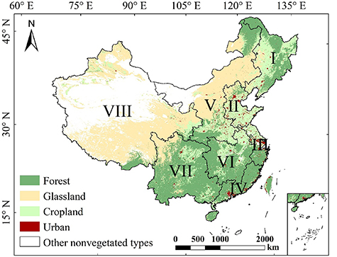
Figure 1. Land cover map of China based on the Moderate Resolution Image Spectroradiometer product in 2014. Different economic regions are indicated: Northeast China (a), Northern Coastal China (b), Eastern Coastal China (c), Southern Coastal China (d), the Middle Reaches of the Yellow River (e), the Middle Reaches of the Yangtze River (f), Southwest China (g), and Northwest China (h).
Download figure:
Standard image High-resolution imageThe land cover information came from the Moderate Resolution Image Spectroradiometer product (MCD12Q1 version 6) at 500 m × 500 m spatial resolution (Friedl and Sulla-Menashe 2015). It was also resampled to a common (1/12)° grid using the land cover type that the most pixels were. The International Geosphere-Biosphere Programme (IGBP) land cover classification provided by the MCD12Q1 product is used in this study. The IGBP classification types are aggregated into five broad land types-forests, grasslands, croplands, urban, and other nonvegetated types. Forests include evergreen/deciduous needleleaf forests, evergreen/deciduous broadleaf forests, and mixed forests. Besides, the closed/open shrublands and woody savannas/savannas are also aggregated into forests due to the small areas of shrublands dominated by woody perennials with 1–2 m height and the woody savanna with tree cover 10%–60% (canopy >2 m). Grasslands are just the grasslands in MCD12Q1 IGBP products. Croplands include croplands and mosaics of natural vegetation and croplands. Urban include urban and built-up lands. Other nonvegetated types include permanent wetlands, permanent snow and ice, barren and water bodies. The LURDs effects on vegetation greenness in the above-mentioned vegetated types were discussed because the obvious LURDs mainly occurred in these areas.
2.2.4. Disentangling the roles of LURDs with the BMA method
The BMA method was used to confirm the roles of LURDs on vegetation greenness. It has been generally used to address the problem of statistical model uncertainty and identify the explanatory variables, which are most likely to determine the dependent variables in many fields (Fernández et al
2001, Horváth 2013, Osada et al
2015, Duc et al
2017). The idea of the BMA lies in estimating the posterior model probabilities that result from Bayes' theorem. Then, the posterior inclusion probability (PIP) and the posterior mean (PM) of explanatory variables were estimated to determine the relative importance and the action directions of explanatory variables based on the posterior model probabilities. Specifically, let us assume that the total number of explanatory variables is K, and the total number of possible individual models is  . We consider numerous different models
  ,...
,... , where
 ![$j \in \left[ {1,{2^K}} \right]$](https://content.cld.iop.org/journals/1748-9326/16/12/124033/revision2/erlac37d2ieqn10.gif) , grouped in the model space M. Thus, the posterior model probability of
, grouped in the model space M. Thus, the posterior model probability of  is obtained as follows (equation (1)):
where y is a dependent variable, Z is the matrix of explanatory variables,  is the marginal likelihood of model
  ,
,  is the integrated likelihood, and
  is the prior model probability. The unit information prior for coefficient priors, and the uniform model priors were used in this work, according to previous studies (Duc et al
2017). Then, the
is the prior model probability. The unit information prior for coefficient priors, and the uniform model priors were used in this work, according to previous studies (Duc et al
2017). Then, the  is obtained by using the Markov chain Monte Carlo Model Composition method. The detailed calculations of
  can be found in Fernández et al (2001) and Zeugner and Feldkircher (2015).
According to the  in equation (1), we compute the PIP as the sum of the models' posterior model probabilities, including the variable k, which denotes the probability that a particular regressor
  is involved in the true model (equation (2)):
where  is the
  (
( ) of a particular regressor
  ,
,  is the posterior probability of
  in
in  .
.
The PM of the distribution of  is as follows (equation (3)):
where  is the averaged coefficient, and
  is the evaluation of the
  from model
  .
.
Eicher et al (2011) and Feldkircher et al (2014) have provided the detailed interpretation of the PIP and PM. The PIP of an explanatory variable with less than 0.5 is characterized as the least weak evidence, while a PIP with larger than 0.5 is characterized as effective evidence. Moreover, it is regarded as weak (0.5–0.75), substantial (0.75–0.95), strong (0.95–0.99), and decisive (0.99+) evidence. In addition, the sign of PM is positive, indicating that the increase in explanatory variables has a positive effect on vegetation greenness, and vice versa.
The contribution of LURDs on the trends in LAIgs (cf section 2.2.2) at the provincial level (31 main provincial administrative regions) was regarded as the dependent variable for the BMA method. Then, we selected the trends in nine potential land-change processes as the explanatory variables in 31 main provincial administrative regions of China from 2000 to 2014, according to the statistical data on land-change processes. The nine statistical land-change processes were detailed descriptions in table S1 (available online at stacks.iop.org/ERL/16/124033/mmedia).
3. Results
3.1. Spatial patterns of greening and browning in different regions
Vegetation greenness, as characterized by the satellite-observed LAIgs, exhibited significant (P < 0.05) increasing trends over 35% of the land area of China from 2000 to 2014 (figure 2). It indicated that a greening pattern was strikingly prominent across China. The notable increase (larger than 0.05  ) in greenness (greening) was generally observed in forested areas of four economic regions: SWC, MRYLR, MRYTR, and SCC (figures 2 and 3).
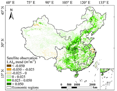
Figure 2. Spatial distribution of the trend in growing season LAI (LAIgs) in China from 2000 to 2014. The LAIgs values represent the mean values of the following satellite products: GLOBMAP LAI, GIMMS LAI3g, GEOV2 LAI, and GLASS LAI (cf section 2.1.1). The significance of trends at the 0.05 level is indicated by the color range with blank areas indicating no trends or nonvegetated areas. Economic regions are shown (thin black lines).
Download figure:
Standard image High-resolution image
Figure 3. The spatial pattern of the contribution of LURDs on significant trends in the growing season LAI in China from 2000 to 2014. White color indicates vegetated areas with no significant trends or nonvegetated areas (cf figure 2). The contribution of LURDs is derived from the difference between scenario S3 and scenario S2 (cf sections 2.2.2 and 2.2.3).
Download figure:
Standard image High-resolution imageIn contrast, the satellite-observed LAIgs trend showed that the LAIgs significantly decrease (P < 0.05) in less than 6% of the land area of China and are sparsely distributed in the two economic regions NWC and ECC (figure 2). This indicated that the areas of vegetation greenness decreases (browning) were relatively small. NWC exhibited that the LAIgs decreased by ⩽−0.025 m2 m−2 yr−1 in its northern and southern parts with the most rural areas. Compared to NWC, a notable decrease in the LAIgs (less than −0.05 m2 m−2 yr−1) occurred in the central part of ECC with a lot of urban land covers (figures 2 and 3).
3.2. Contribution of LURDs to the LAIgs trends
The nationally averaged LURDs resulted in a significant (P < 0.05) increase in China's LAIgs (figure 3). The increased magnitude was  m2 m−2 yr−1, which was approximately 7.9% of the nationally averaged LAIgs trend estimated by satellite-observed datasets (
 ) (figures 2 and 4).

Figure 4. (a) The trends in forest area change (FAC), the area changes of forest biodisasters and fire disasters (AFBF), urban area change (UAC), urban green space (UGS), grassland area change (GAC), the area changes of grassland biodisasters and fire disasters (AGBF), and cropland area change (CAC) in eight economic regions. (b) The trends in total crop-yield change (CY) and the number of total livestock (TL) in eight economic regions. Only changes that show a significant trend at the 0.05 level are shown (cf section 2.2.3).
Download figure:
Standard image High-resolution imageThe trends in vegetation greenness that were attributed to LURDs were then further estimated at the eight economic regions and on a per-pixel basis (table 3 and figure 3). The positive and negative differences between scenario S3 and scenario S2 indicated the positive and negative effects of LURDs on greenness, respectively. We then classified the model differences in three levels using the following values as threshold values: the average LURDs contribution in the trend of the LAIgs  and the observed average LAIgs trend
  . The absolute difference between scenario S3 and scenario S2 was higher than the observed average LAIgs trend, which was regarded as a highly significant effect. The absolute difference was less than the average LURDs contribution, which was characterized as a mildly significant effect. The absolute difference value between
  and
and  was characterized as a moderately significant effect. Generally, the LURDs effects on the LAIgs showed a strong spatial variation across the mainland of China (table 3 and figure 3).
Table 3. The area fractions of LURDs effects on growing season LAI trends.
| Significant positive effect | Significant negative effect | |||||||
|---|---|---|---|---|---|---|---|---|
| Regions | High | Moderate | Mild | Total | High | Moderate | Mild | Total |
| NEC | 9.75% | 7.46% | 0.03% | 17.24% | 3.33% | 0.00% | 3.28% | 6.61% |
| NCC | 3.89% | 4.35% | 0.00% | 8.24% | 4.59% | 0.00% | 4.03% | 8.62% |
| ECC | 4.52% | 10.42% | 0.43% | 15.37% | 5.66% | 0.05% | 3.43% | 9.14% |
| SCC | 9.46% | 26.27% | 0.09% | 35.82% | 3.06% | 0.12% | 3.79% | 6.98% |
| MRYLR | 4.73% | 11.71% | 3.12% | 19.56% | 1.74% | 0.80% | 2.32% | 4.87% |
| MRYTR | 13.03% | 18.75% | 0.00% | 31.79% | 3.91% | 0.00% | 4.19% | 8.11% |
| SWC | 18.38% | 14.07% | 0.02% | 32.47% | 5.23% | 0.02% | 2.04% | 7.29% |
| NWC | 1.63% | 6.97% | 3.89% | 12.48% | 3.12% | 7.85% | 7.81% | 18.78% |
| Total | 6.51% | 10.39% | 2.21% | 19.11% | 3.39% | 3.46% | 4.98% | 11.83% |
Our results suggested that LURDs had led to significant (P < 0.05) increases of the LAIgs over 19.11% of the land area of China (table 3). The significantly positive LURDs effects were mainly distributed in SCC, SWC, MRYTR, MRYLR, and NEC, which had dense forest cover with part cropland cover (figures 2, 4, and S1(a)). SCC had the greatest area fractions (up to 35.82% of its corresponding area) of significant positive effects of LURDs on the LAIgs trends, following by SWC (32.47% of its corresponding area) (table 3). However, SWC and NEC were dominated by the high significant positive effects of LURDs on the LAIgs trends. SCC, MRYTR, and MRYLR were dominated by the moderate significant positive effects of LURDs on LAIgs trends. Meanwhile, the statistical data on land-change processes showed that SWC had increasing trends in forest areas with a rate of 0.0090  , which was higher than SCC, MRYTR, and MRYLR (figure 4(a)). NEC experienced the largest significant increase in crop yield (figure 4(b)). These suggested that the effects of LURDs on vegetation greening were primarily related to the increases in forest area (afforestation) and improved crop yield (advanced agriculture), but the effect of the latter was just observed in parts of cropland-dominated areas, which was far less than that of the former.
Compared to the positive effects of LURDs on the LAIgs, the area of LURDs negative effects on LAIgs trends was relatively small at a national scale. It had led to significant decreases in LAIgs over 11.83% of China's land (table 3). The decreases in LAIgs trends due to LURDs mainly occurred in ECC and NCC with much urban cover, in parts of NWC with much grassland cover, and sporadically occurred in MRYTR and SWC with forest cover (figures 2 and 4). NWC (18.78% of its corresponding area) had greater area fractions of significant negative effects of LURDs on LAIgs trends than other economic regions, following by ECC and NCC (9.14% and 8.62% of its corresponding area, respectively). However, ECC and NCC were dominated by large significantly negative effects of LURDs on LAIgs trends, while NWC was dominated by the moderate and mild significant negative effect of LURDs on LAIgs trends. Besides, MRYTR and SWC had the area fractions of significant negative effects of LURDs on LAIgs trends with 8.11% and 7.29%, respectively, in which large significant negative effects of LURDs on the LAIgs trends were dominated. Meanwhile, the statistical data on land-change processes showed that ECC had significantly increasing trends in urban areas, with the largest rates of 0.00145 yr−1, followed by NCC (figure 4(a)). MRYTR experienced the largest significantly increasing trend (0.00059 yr−1) in areas of forest biodisasters and fire disasters (figure 4(a)), whereas SWC had the affected grassland areas by biodisasters and fire disasters with the largest significantly increasing trend (0.00195 yr−1). Besides, NWC had the largest increasing trend in total livestock (170.5  ) (figure 4(b)). These results indicated that LURDs effects on vegetation browning were mainly associated with the increased urban area (urbanization), biodisasters and fire disasters of forests, biodisasters and fire disasters of grasslands, and increased total livestock (overgrazing). However, the magnitude of urban expansion on vegetation browning was larger than that of these latter factors, although the urban area in China was relatively small, accounting for approximately 1.4% of the land area of China.
3.3. The roles of LURDs on vegetation greenness
To disentangle the roles of the main LURDs on the observed greenness changes in China, we introduced a BMA method based on two scenario simulations and statistical data on land-change processes. As shown in table 4, forest area change, urban green space area, crop yield, grassland area change, and crop area change showed that the signs of PM are positive. It indicated that the five abovementioned changes had positive effects on vegetation greenness. Moreover, the PIP of forest area change was 0.998, and China exhibited significant and large increasing trends in forest areas in eight economic regions (figures 2 and 5(a)). This indicated that afforestation had a decisive role in explaining vegetation greening in China. The PIPs of urban green space area, crop yield, grassland area change, and crop area change were less than 0.5, and they had significant increasing trends in most economic regions (figure 4). This indicated that urban greening, advanced agriculture, and grassland restoration had the least effective roles in explaining vegetation greening.

Figure 5. Changes in growing season LAI (m2 m−2) from 2000 to 2014 averaged for four different land cover types in China (cf section 2.2.3). Trends are shown for different land use classes, indicating the effect of changes within different land-use types on the corresponding average trends in satellite-observed LAIgs. Land-use specific trends are computed by ecosystem process model simulation (for details seeing section 2.2.3). Significant trends at the 0.05 level are indicated (*) other factors.
Download figure:
Standard image High-resolution image
Table 4. The determinable roles of LURDs on vegetation greenness: Bayesian model averaging evidence.
| Resources and environmental statistics variables | PIP | PM |
|---|---|---|
| Forest area change | 0.998 | 0.477 |
| Urban area change | 0.997 | −0.753 |
| Area change of forest biodisasters and fire disasters | 0.848 | −0.237 |
| Urban green space | 0.316 | 0.111 |
| Area change of grassland biodisasters and fire disasters | 0.273 | −0.035 |
| Crop yield | 0.225 | 0.025 |
| Total livestock | 0.183 | −0.012 |
| Grassland area change | 0.179 | 0.011 |
| Cropland area change | 0.165 | 0.002 |
Notes: PIP indicates posterior inclusion probability. PM indicates a posterior mean.
In contrast, the PMs of urban area, the biodisasters and fire disasters area of forests and grasslands, and the total livestock indicated that the increases in these drivers had negative effects on vegetation greenness. Moreover, the PIP of urban area and the area of forest biodisasters and fire disasters were larger than 0.5, indicating that they were effective land–change processes that explain vegetation browning. The PIP of urban area change was 0.997, and the urban area of China showed significantly increasing trends. This indicated that urbanization had a decisive role in vegetation browning. The forest biodisasters and fire disasters had a substantial role in vegetation browning, with a PIP = 0.848, resulting from significant increasing trends in the area of forest biodisasters and fire disasters across forest-dominated regions such as MRYTR, SWC, and MRYLR (figures 2 and 5(a)). The PIPs of the total livestock and the area of grass biodisasters and fire disasters were less than 0.5, and they had significant increasing trends in some regions with excessive grassland cover such as NWC (figures 2 and 5). The phenomenon suggested that biodisasters and fire disasters or overgrazing in grassland areas had the least effective roles in explaining vegetation browning of the whole China mainland.
4. Discussion
4.1. The vegetation greenness trend in China
Our results showed that the spatial pattern of vegetation greenness change based on satellite measurements from 2000 to 2014, which was consistent with previous studies suggesting considerable local effects of LURDs on vegetation greenness (Liu et al 2016, Hua et al 2017, Chen et al 2019b, Miao et al 2020). The most notable vegetation greening was generally distributed in parts of SWC, MRYLR, MRYTR, and SCC. These regions are important forest-dominated areas with a series of large-scale conservation programs (figures 2 and S2) and have suitable climates for vegetation growth (Feng et al 2016, Li et al 2017, Deng et al 2017a). For example, two unprecedented conservation actions—the Natural Forest Conservation Program (NFCP) and the Grain to Green Program (GTGP) have been taken in China since 1999, which cover four out of five provincial administrative regions (Liu et al 2008). The notable vegetation browning was generally distributed in parts of NWC with rural areas characterized as ecological vulnerabilities (Liu et al 2008) and in parts of ECC with high urbanization. Additionally, significantly increased trends (0.0089 m2 m−2 yr−1) in vegetation greenness were observed at the national scale from 2000 to 2014. Such general trends at the national scale were slightly larger than that (0.0070 m2 m−2 yr−1) of the period from 1982 to 2009 (Piao et al 2015). Meanwhile, the patterns of satellite-observed LAIgs trends were consistent with the previous study (Piao et al 2015). It suggested that the trend in vegetation greening has continued in China during 2010–2014.
4.2. Local contributions of land use related-drivers on vegetation greenness
The IPM factorial simulations showed that the general effect of LURDs on vegetation greening was relatively limited if spatially average for China. There was almost identical evidence that the average effects of LURDs on observed LAI trends are relatively small on hemispherical or global scales (Zhu et al
2017, Chen et al
2019b). Moreover, such a positive effect was just 9.6% of that caused by both  (figure 5). It was consistent with previous studies that the enhanced
  fertilization and climate change are the dominant causes of vegetation greening at a global or regional level (Piao et al
2015, Mao et al
2016, Zhu et al
2016, 2017, Chu et al
2019).
fertilization and climate change are the dominant causes of vegetation greening at a global or regional level (Piao et al
2015, Mao et al
2016, Zhu et al
2016, 2017, Chu et al
2019).
The effects of LURDs on vegetation greenness exhibited a strong spatial heterogeneity on a per-pixel basis (figure 3). The area with positive LURDs effects on greenness was overall greater than that with negative effects. Afforestation had a notable positive effect on vegetation greenness, widely distributed in densely forested areas in SCC, SWC, MRYTR, and MRYLR. It was consistent with previous results highlighting that the greening trend is the largest in southern China due to increased forest cover (Li et al 2018c). A series of regional and national afforestation projects have been developed and implemented across China to restore the degraded environment (Li et al 2019). At least three afforestation projects are implemented in the above-mentioned four economic regions, including GTGP, NFCP, and the corresponding regional forest projects (figure S2). Two of the four economic regions, SWC and MRYLR, have the largest cumulative afforestation area (figure S1(b)). Besides, timber forests (such as eucalyptus) are widely planted in the afforestation projects of the four regions. This has notable effects on the vegetation greening due to its specific characteristics as being fast-growing, highly adaptable, and fruitful (Liu et al 2017). Moreover, large significantly positive effects of LURDs were mainly distributed in parts of SWC with forest cover where the cumulative afforested areas of timber forests were larger than other economic regions. Meanwhile, large significantly negative effects of LURDs were sporadically distributed, mainly because of the negative effects of biodisasters and fire disasters of forests. It means that forest biodisasters and fire disasters generally pose some serious threats to vegetation growth (Wen et al 2016). However, the area and magnitude of afforestation effects were far greater than that of forest biodisasters and fire disaster effects (figure 3). Advanced agriculture could also lead to vegetation greening, mainly distributed in parts of cropland-dominated areas in NEC (figures 2 and 4). Based on the China Statistical Yearbooks from 2000 to 2014, the total crop yield had increased by 31.4%, and the total cropland area only increased by 3.9%. However, the effect of advanced agriculture on vegetation greening was not notable, probably resulting from the inconsistency of the various crops growing season in different regions (Wang et al 2017).
In contrast, urbanization had an important effect on vegetation browning. It was mainly distributed in densely urban areas in ECC and NCC, where the significantly increasing trends in urban areas were experienced from 2000 to 2014 (figure 4(a)). Although these regions had generally significantly increasing trends in the urban greenness space area, the negative effects of urbanization were far outweighed by such positive effects (figure 4(a)). This result is generally consistent with the findings of prior studies (Wu et al 2014, Li et al 2018b). Additionally, the biodisasters and fire disasters of grasslands and overgrazing also had local effects on greenness in grassland-dominated areas, but it had limited effects if spatially average for China (table 3 and figure 3). It was likely that the negative effects of grassland biodisasters and fire disasters, and overgrazing might be outweighed by the implementations of grassland restoration projects in China over recent years (Guo et al 2018). For example, the implementation of the Returning Grazing Land to Grassland Program (RGGP), which aims to alleviate grazing pressure through grazing exclusion, has obtained some achievements over the past two decades (Deng et al 2017b, Zhang et al 2018).
To further appreciate the contrasting effects of afforestation and urbanization on vegetation greenness, we compared the effects of LURDs and both  on observed LAIgs trends at four broad land types at the national (figure 5) and economic region (figure S3) scales. The magnitudes of the LURDs effects on vegetation greenness varied in different areas. However, LURDs related to afforestation and urbanization largely altered vegetation greenness at the national and regional levels. Compared to the regional scale, afforestation and urbanization made noticeable effects on vegetation greenness at the national scale. The residual LURDs effects were relatively limited, accounted for less than 8% of the corresponding observed greenness changes at the national scale (figure 5).
As shown in figure 5, LURDs related to increased forest area had a larger effect on observed greening in the forest areas than that in the cropland areas and the other land cover areas. Like previous studies of (Li et al
2018c, Chen et al
2019b), the increased forest area associated with large-scale afforestation should effectively result in vegetation greening. However, our study gave out a quantitative assessment of such a positive greening effect of afforestation in the forest area as 27%. And it only accounted for about half of the positive effects of both  . It was likely that the negative effects of the damaged forest by fire, pests, and rodents may partly offset the positive effects of afforestation.
Compared to forest areas, LURDs in the urban areas exhibited the largest negative effect on vegetation greenness, while the magnitude of such negative effects was slightly less than the positive effects of afforestation on greenness (figure 5). Because the satellite-observed average LAIgs trend was negative in the urban area, the positive  effect had a 70.5% offset to the vegetation browning. If there was not the impact of
  and other factors, the LURDs could cause approximately two times vegetation browning relatively to the satellite-observed average LAIgs trends in the urban area. This suggests that the magnitude of the negative effects of LURDs is about three times the positive effects caused by the
  . It highlights that urbanization has important effects on vegetation browning relative to the dramatic urbanization undergone in China over the last 15 years (Li et al
2018a, 2018b).
. It highlights that urbanization has important effects on vegetation browning relative to the dramatic urbanization undergone in China over the last 15 years (Li et al
2018a, 2018b).
The BMA evidence made up for the deficiency of the IPM factorial simulations. It confirmed that afforestation had a decisive role in leading to vegetation greening, although the biodisasters and fire disasters of forests have substantial effects on vegetation browning. China experienced significant increasing trends in forest areas due to the widespread implementation of several afforestation projects (figure 4(a)). In contrast, urbanization had decisive effects on vegetation browning. The reason was likely because China experienced significant increasing trends in urban area changes related to rapid urban expansion since the 1990s (Liu et al
2014, Zhou et al
2016, He et al
2017, Sun and Zhao 2018). Additionally, advanced agriculture, urban greening, grassland restoration, overgrazing, and grass biodisasters and fire disaster made relatively small contributions to China's vegetation greenness at the national scale. It was likely that vegetation greenness was more susceptible to both  or other factors in the cropland and grassland areas (figure 5).
In summary, this study highlighted the importance of the combination between process-based ecosystem models and the BMA statistical method. The former was effective in separating the contributions of LURDs and biogeochemical factors. They could quantify the individual contributions of LURDs to the observed greening trend on a per-pixel basis, at the national and regional levels, and various vegetation cover types. Meanwhile, the latter based on the statistical data could characterize the roles of LURDs such as afforestation, urbanization, and agricultural management at statistical levels.
The results indicated that afforestation and urbanization as the two main types of LURDs had decisive roles in vegetation greening and browning in China, respectively. On the one hand, a series of ambitious revegetation programs have been successfully implemented in China to restore degraded ecosystems and mitigating climate change. Already 62 million hectares of current forests have been until 2008, occurring for the largest percentage of the world's afforestation, according to the seventh national forest resource inventory report (2004–2008) (Deng and Shangguan 2017, Li et al 2018c). The growth of newly planted forests could make further greening more significant. For example, Chen et al (2019b) demonstrated that China is one of the countries that lead in the greening of the world through human land-use management from 2000 to 2017. Other recent studies attest to the success of these revegetation programs in terms of restoring degraded ecosystem (Feng et al 2016), lowering the surface temperature (Yu et al 2020), improving carbon sequestration (He et al 2020), and providing biofuel for bioenergy production (Menz et al 2013), but a strain on water resources in arid and semi-arid environments has also noted (Tang et al 2018, Bai et al 2020). Furthermore, the Chinese government is projected to expand afforestation programs (Chen et al 2015). It can be expected that the afforestation would have significant effects on vegetation greening over the next several years. In addition to China, other regions of the world have also promoted afforestation in the present and future (Duque-Lazo et al 2018, Kemena et al 2018, Odoulami et al 2018, Yosef et al 2018, Zhang et al 2021). It is therefore believed that afforestation is a profound factor affecting vegetation greening and should be highlighted in the design and implementation of local ecosystem management plans.
On the other hand, the urbanization rate (urban population in China as a percentage of the total population) raised from 36.22% in 2000 to 54.77% in 2014, according to the National Bureau of Statistics of China. China's urbanization rate is expected to hit 80% by 2050 (United Nations and Social 2018). It suggested that the rapid urban expansion of China cannot be ignored by ecosystem management. Other current studies demonstrate that urban expansion reduces regional net primary productivity (NPP) due to the LURDs-induced direct effect (Guan et al 2019, Wen et al 2019). The decreases in NPP due to the urban expansion from cropland accounted for 63.02% of the total loss in NPP in mainland China, which may threaten the food security of China (Li et al 2018b). Meanwhile, other countries across the world have also experienced growing urbanization rates and their effects on vegetation dynamics over the last few decades (Cai et al 2019, Yao et al 2019, Nathaniel et al 2020). Large urbanization is projected to continue in the future across these countries, particularly in developing countries (United Nations and Social 2018). Thus, the local effects of urbanization on vegetation browning become greater with the accelerated process of urbanization and should be given increased attention at regional to global scales.
There are some uncertainties and limitations regarding the performance of the ecosystem model results in simulating the LURDs effects on vegetation greenness, despite the great efforts that have been undertaken to optimize the robustness of the ecosystem models. Future work needs to further improve the reliability of our results through the comparative analysis of our methodology and other novel methodology. For example, the novel approach to estimate LURDs effects is directly based on the difference between historic and current land cover maps and could also be considered in vegetation change attribution analyses (Pei et al 2013, Li et al 2018b). The simulation scenes of forest age, agricultural irrigation, and grazing management also need to be considered in future ecosystem models to explore the roles of LURDs on vegetation greenness.
5. Conclusions
This study disentangled the role of different LURDs on vegetation greenness across China from 2000 to 2014 through combining process-based ecosystem models and the BMA statistical method. Results showed vegetation greening over 35% of the land area of China, whereas less than 6% of the country exhibited vegetation browning. LURDs exhibited considerable local effects on vegetation greenness, although these effects were relatively limited (approximately 7.9%) at the national scale. Afforestation and urbanization as the two main types of LURDs had decisive roles in vegetation greening and browning in China, respectively. The area fraction of afforestation effects on greening was more than 30% in SCC, MRYTR, and SWC with massive forest planting programs. Although it was offset by forest biodisasters and fire disasters (with substantial roles), afforestation still explained 27% of the observed greening trends in the forests of China. In contrast, urbanization caused 199% of the browning trends relative to observations from the urban area, which was almost three times as much as the positive effects of both climate change and CO2 fertilization. The residual LURDs effects accounted for less than 8% of the corresponding observed greenness across China. Future studies could be further extended to the vegetation greenness worldwide and become useful in assisting better global ecosystem management planning.
Acknowledgments
This study was jointly supported by the National Natural Science Foundation of China (General Program) under Grant 42171381, the National Key Research and Development Program of China under Grant 2018YFC1506506, the National Key Research and Development Program of China under Grant 2017YFB0503905, and State Scholarship Fund of CSC 201704910106. We thank the TRENDY modeling group for providing the TRENDY v4 and v5 model data.
Data availability statement
The data generated and/or analysed during the current study are not publicly available for legal/ethical reasons but are available from the corresponding author on reasonable request.