

Abstract
London introduced the world's most stringent emissions zone, the Ultra Low Emission Zone (ULEZ), in April 2019 to reduce air pollutant emissions from road transport and accelerate compliance with the EU air quality standards. Combining meteorological normalisation, change point detection, and a regression discontinuity design with time as the forcing variable, we provide an ex-post causal analysis of air quality improvements attributable to the London ULEZ. We observe that the ULEZ caused only small improvements in air quality in the context of a longer-term downward trend in London's air pollution levels. Structural changes in nitrogen dioxide (NO2) and ozone (O3) concentrations were detected at 70% and 24% of the (roadside and background) monitoring sites and amongst the sites that showed a response, the relative changes in air pollution ranged from −9% to 6% for NO2, −5% to 4% for O3, and −6% to 4% for particulate matter with an aerodynamic diameter less than 2.5 μm (PM2.5). Aggregating the responses across London, we find an average reduction of less than 3% for NO2 concentrations, and insignificant effects on O3 and PM2.5 concentrations. As other cities consider implementing similar schemes, this study implies that the ULEZ on its own is not an effective strategy in the sense that the marginal causal effects were small. On the other hand, the ULEZ is one of many policies implemented to tackle air pollution in London, and in combination these have led to improvements in air quality that are clearly observable. Thus, reducing air pollution requires a multi-faceted set of policies that aim to reduce emissions across sectors with coordination among local, regional and national government.
Export citation and abstract BibTeX RIS

Original content from this work may be used under the terms of the Creative Commons Attribution 4.0 license. Any further distribution of this work must maintain attribution to the author(s) and the title of the work, journal citation and DOI.
1. Introduction
Air pollution exposure is the second leading cause of noncommunicable diseases and ambient air pollution was estimated to cause 4.2 million premature deaths worldwide in 2016 (World Health Organization 2018). The transport sector is one of the main sources of air pollutant emissions and consequently various interventions have been implemented to mitigate its air pollution impacts. The Euro vehicle emissions standards were first introduced in 1992 (Directive 91/441/EEC) and they have been progressively tightened to reduce EU-wide emission levels of new vehicles. Pricing schemes have been implemented to internalise external environmental costs with congestion pricing, for example, used to reduce congestion and/or air pollution, implemented in Singapore, London, Stockholm, and Milan (Croci 2016). Low Emission Zones (LEZs) are another common approach, with different designs of standard based on fuel type, vehicle type, minimum emission standards, and operating time (Holman et al 2015). Vehicles entering the LEZ are banned (such as in cities in Germany) or required to pay an extra cost (such as in London) if they cannot meet the required standard (Obrecht et al 2017).
On 8 April 2019, London introduced the world's most stringent emissions zone, the Ultra Low Emission Zone (ULEZ), to accelerate compliance with the EU air quality standards. Compared with the London LEZ (introduced in 2008), which targets heavy-duty vehicles across most of Greater London, the ULEZ affects all types of motorised vehicles but over a smaller area of central London. When introduced, the ULEZ coincided with the Congestion Charge Zone (CCZ) and it is active 24 h a day, 7 d a week. On top of the congestion charge, vehicles entering the ULEZ are required to pay a daily charge if they fail to meet the required emission standards. The ULEZ replaced the Toxicity Charge (T-Charge), which was effective from October 2017 in central London (Greater London Authority 2019). Compared with the T-charge, the ULEZ is operational for more time, applies a higher charge, and requires stricter minimum emission standards (Greater London Authority 2017, 2019). The Greater London Authority (2019) estimated a 29% reduction in roadside NO2 concentrations in central London from July to September 2019 attributable to the ULEZ. While the ULEZ area is confined to central London, the majority of traffic entering the ULEZ comes from outside the zone and the policy is expected to encourage the upgrade of vehicle fleets in a wider area and consequently affect vehicle emissions across the city (Transport for London 2021).
The effectiveness of transport interventions at improving air quality can be highly variable, spatially heterogeneous (Kelly et al 2011, Holman et al 2015), and time-dependent (Percoco 2013). Behavioural changes in response to a transport intervention can evolve, consequently dynamically affecting air pollution emissions. Factors contributing to the dynamic response in activities include the anticipation effect (Ellison et al 2013, Ciccone 2018), and the delay in response and/or gradual adaptation afterward (Börjesson et al 2012, Gallego et al 2013). In addition, as a city is a complex network, behavioural changes may not be restricted within the area where the transport intervention is actually implemented, indicating a spatial spillover effect of the intervention (Wolff 2014, Green et al 2016).
To inform future development strategies, it is important to quantify the effects of transport interventions on air quality. Causal inference methods can be used to evaluate the causal relationship between a putative cause (such as a transport intervention) and an outcome (such as air quality level). Identification of a causal relationship goes beyond mere quantification of statistical association or correlation in the sense that it seeks to measure the direct net effect of an intervention on an outcome through all possible pathways (Pearl 2010, Altman and Krzywinski 2015). A transport intervention is generally targeted to specific areas of interest (non-randomised) and some common causes exist between transport activities and air quality levels including weather conditions and seasonality effects (confounders), which present challenges to identifying the causal impacts of a transport intervention on air quality (Grange and Carslaw 2019, Brancher 2021).
Several previous studies have used causal inference methods to conduct ex-post assessments of the air quality effects of transport interventions. Examples include congestion/road pricing (Percoco 2013, Gibson and Carnovale 2015), driving restrictions (Davis 2017, Zhang et al 2017), and changes in public transport supply (Gendron-Carrier et al 2018, Ma et al 2021). Difference-in-differences (DID) and regression discontinuity design (RDD) are two main causal inference methods used in previous studies. Both of them can be applied to non-randomised interventions, yet they have different assumptions: RDD assumes the treatment is assigned by the value of a forcing variable on either side of a threshold, whereas DID requires the definition of two groups (treatment group and control group) and two time periods (before and after the intervention), and assumes that only the treatment group in the after-intervention period is exposed to the treatment (Imbens and Wooldridge 2009). In this paper, we interchangeably use the terms 'intervention' and 'treatment'.
This study aims to provide an ex-post assessment of the London ULEZ, using a sharp RDD model, to quantify the causal effects on air quality at different monitoring sites. As the world's most stringent emissions zone, this ex-post assessment contributes to the evidence base for future transport interventions that aim to improve air quality. Details omitted from the main text of this paper are included in the supporting information (SI), as referenced.
2. Materials and methods
The methodology of this paper mainly follows Ma et al (2021) with further improvements. Ma et al (2021) proposed a methodology combining meteorological normalisation, change point detection (CPD), and a sharp RDD to evaluate the causal air quality impacts of a transport policy. With an explicit start time, the London ULEZ is conceptually consistent with the sharp regression discontinuity in time (RDiT) approach where the start of the ULEZ is regarded as the threshold.
First, meteorological normalisation is applied to control the important baseline covariates (meteorological variables and seasonality variables) that may violate the continuity assumption of a valid RDD. Meteorological variables considered in this process include temperature, wind speed, wind direction, atmospheric pressure, relative humidity, rainfall, and Monin-Obukhov length. Seasonality variables contain the hour of the day, day of the week, and day of the year. A time variable is also included to represent the long-term trend of the concentrations. A normalised air pollutant concentration time series is derived by removing the variation in the observed concentrations that can be explained by meteorological conditions and seasonality effects. Further details are included in SI section S1 (available online at stacks.iop.org/ERL/16/124001/mmedia). The relative importance and partial dependence of the above covariates in predicting concentrations are also discussed in SI section S1. The rank of relative importance for the model of nitrogen oxides (NOx ) concentrations at a site of example is generally aligned with the result in Carslaw and Taylor (2009).
Secondly, CPD is conducted to detect the changes in the normalised air pollutant concentration time series. The detected change points are used to test the discontinuity in the normalised concentrations (outcome) around the threshold to justify the use of a sharp RDD (see section 2.2.1); they are also used to truncate the normalised concentration time series into segments to support the research period specification of sharp RDD models (see section 2.2.2). Compared with Ma et al (2021), the CPD in this paper detects structural changes instead of mean-shifts. A change in the slope of the linear trend and/or an abrupt discontinuity in the normalised concentration time series is identified as a structural change, see details in SI section S2. As the RDiT is interested in the discontinuity in the outcome at the threshold and its evaluation relies on trend function approximation on either side of the threshold (Lee and Lemieux 2010), detecting structural changes is conceptually more consistent with the RDiT approach.
Thirdly, a sharp RDD model (see section 2.2) is specified on the normalised air pollutant concentration time series at individual monitoring sites. The parameters estimated from the sharp RDD model are used to derive the causal effect of the ULEZ (see section 2.2.3). Lagged dependent variable(s) are incorporated in the sharp RDD model to account for the autocorrelation in the outcome variable. Newey-West standard errors are computed to account for the autocorrelation in the regression residuals. To account for any anticipation, adaptation, or delay in response to the ULEZ, we specify the main model as a 'donut' RDD to give a better estimation of the full intervention effect (see section 2.2.2). While a regular RDD uses all data in the research period to estimate the effect, like in Ma et al (2021), a donut RDD excludes the data in the vicinity of the threshold.
The interaction among different steps of the methodology is illustrated in figure 1.
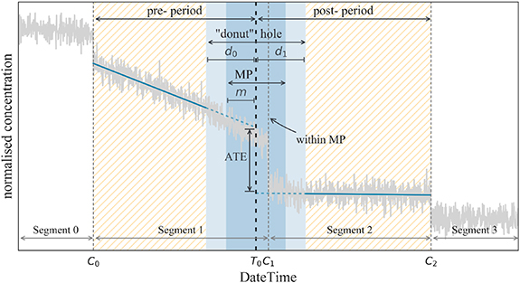
Figure 1. Graphical summary of methodology. The normalised air pollutant concentration time series (grey line) is illustrated with the detected change points  (grey; dashed lines). The margin period (MP) and the 'donut hole' are shaded around the start of the ULEZ
  (threshold) (black; dashed line). The size of MP and the donut hole are labelled with corresponding length parameter(s), where
  for MP, and
  and
and  for the donut hole. The data within the orange hatched area are used for RDD model fitting. The average treatment effect (ATE) is given by the difference in intercept at
  . The intercepts are estimated based on the trend function approximation (blue line) on either side of
  .
.
Download figure:
Standard image High-resolution image2.1. Case study specification and data description
To quantify the causal air quality effects of the London ULEZ across London, we specify a sharp RDD model at individual air quality monitoring sites, for regulated pollutants including nitrogen dioxide (NO2), ozone (O3), and particulate matter with an aerodynamic diameter less than 2.5 μm (PM2.5) and 10 μm (PM10). NOx (NO + NO2) and total oxidant (OX, OX = NO2 + O3), while not regulated, are also included to provide additional insight. The ULEZ was implemented from 2019-04-08 00:00, which we define as the start of the intervention. Data from 2016-01-01 (39 months before the ULEZ) to 2020-01-31 (9 months after the ULEZ) are used. The data after 2020-01-31 is not included to avoid possible changes in activity in response to the COVID-19 pandemic. The research area is defined by the geographical extent of Greater London to consider a potential spatial spillover effect of the ULEZ.
Roadside, background, and kerbside monitoring sites are distinguished in our analysis. A roadside monitoring site is generally installed within 1–5 m of a busy road at breathing height to represent roadside public exposure. A background monitoring site is located away from major emission sources and broadly representative of public exposure at the town-wide or city-wide level. A kerbside site is generally installed within 1 m of the kerb of a busy road and is dominated by road traffic emissions (Greater London Authority 2018). As kerbside sites are not typical of public exposure and fewer in number, we mainly focus on the ULEZ's effects on roadside and background concentrations, with estimates of the effects on kerbside concentrations included to further understand the change in traffic emissions. A monitoring site is included in the analysis for a particular pollutant only if the data quality criteria are met (see SI section S11).
Hourly air pollutant concentrations at monitoring sites are downloaded from the open-source data in the London Air Quality Network (Imperial College London 2018). Seventy-nine monitoring sites (background: 28; roadside: 43; kerbside: 8) are included in the study in total after the application of the data quality criteria. Hourly meteorological observations are from the Integrated Surface Database and the Radiosonde Database of the U.S. National Oceanic and Atmospheric Administration (NOAA) (NOAA 2008, 2020). Further details on the data description are included in SI section S11.
We note that the private hire vehicle (PHV) exemption from the congestion charge was removed on the same day as the introduction of the ULEZ. Therefore, it is difficult to separate the effects of these two interventions based on air quality observations, however, the impact of removing the PHV exemption was estimated to be a 1% reduction in road traffic in the CCZ (Transport for London 2018).
2.2. Sharp RDD model
We now specify the causal inference process to estimate the causal air quality impacts of the London ULEZ.
2.2.1. Response identification
To justify the use of a sharp RDD, it is necessary to test the discontinuity in the outcome at the threshold (Lee and Lemieux 2010). Instead of strictly checking at the threshold, we introduce an MP around the start of the ULEZ  (threshold) to consider the potential uncertainties in the stochastic process in previous steps (cf figure 1). The length parameter
  reflects the expectation of the uncertainty. A normalised concentration time series is considered to have responded to the ULEZ if it has detected at least one change point that lies within the MP. A sharp RDD model is then specified where a monitoring site showed a response.
2.2.2. Research period specification
To mitigate influences from potential unobservable confounders and unrelated interventions, we truncate the normalised concentration time series into segments based on the detected change points; only the data in the segments that are near  are used to estimate the RDD model (cf figure 1). Further details on research period specification and the length of pre- and post-periods specified in the case study are summarised in SI section S3.
Within the research period, a donut RDD is specified following Barreca et al (2011), where the data within the donut hole are excluded from RDD model estimation (cf figure 1). The length parameters  and
and  denote the length of the donut period either side of the intervention. To validate the use of the donut RDD in this study, we compared the effect estimates using both the donut and regular RDD settings (see SI section S5). Effect estimates under these two settings would be similar if a transition of the intervention effect does not exist or is not obvious. However, for most of the air pollutants analysed in this study, we found significantly different effect estimates under these two settings, indicating the existence of a transition period. Furthermore, the proportion of vehicles that comply with the ULEZ minimum emission standards (compliance rate) within the zone continued to increase in the months following the launch of the ULEZ (Greater London Authority 2020a), which provides real-world evidence for a lagged effect.
In the causal inference process, it is necessary to determine the MP and the donut hole. For simplicity, we set the donut hole as symmetric and of the same length as the MP, that is  . A range of candidate lengths is determined based on analysing the timing of the response. The causal inference process is conducted individually with each candidate length. A sensitivity analysis is performed on the estimated effects at individual monitoring sites (see SI section S6). The optimal length is determined based on the sensitivity analysis and we select the group of effect estimates which are less sensitive to the change in the value of
  ,
,  , and
, and  , see SI section S6. An alternative selection method considering the model performance is also discussed in SI section S6.
2.2.3. Model specification and estimation
Normalised hourly concentrations are used to calculate 24 h averages to reduce noise in the time series. The model is based on a sharp RDD in time with the start of the ULEZ being the threshold, following Ma et al (2021) with further details in SI section S4. By incorporating the lagged dependent variable(s) in the model, the total effect of the ULEZ,  , is derived by calculating the sum of the impact from the current daily period and the stacked impact from the previous (lagged) daily periods (Henderson 1996); the derivation is based on the estimated coefficients from the sharp RDD model including the difference in intercept at
  (cf figure 1) and the autocorrelation features of the outcome variable, see SI section S4. By specifying the dependent variable as the natural logarithm transformation of the outcome variable, the
  estimate can be interpreted as the percentage change in daily average concentration caused by the ULEZ (Benoit 2011).
The main model is estimated by ordinary least squares with Newey-West standard errors. To represent the uncertainty in the estimation of  , we compute the interval estimate of
  following a Monte Carlo simulation in Ma et al (2021). The statistical significance of
  at the 10%, 5%, and 1% levels are respectively determined if the corresponding confidence interval (CI) does not straddle zero. In this paper, we mainly discuss the statistical significance of
  at the 10% level.
2.2.4. Regional mean
To compare the ULEZ's effects on air quality within the ULEZ, outside the ULEZ, and across London, we aggregate the effect estimates for each pollutant at different monitoring sites using the bootstrapping approach described in Ma et al (2021). We distinguish between roadside, background, and kerbside sites and additionally present results for aggregation of only those sites where a response was detected.
3. Results and discussion
We now discuss the ULEZ's effects on air quality concerning the concentrations of different air pollutants, with a focus on roadside and background sites. The results for kerbside concentrations are briefly discussed in this section with further details in SI section S14. The timing of the response to the ULEZ is discussed in section 3.1. The estimated effects on different air pollutants are discussed in section 3.2, with a focus on NOx and NO2. Effect estimates for O3 and PM2.5 concentrations were generally less significant, and those for PM10 appear to have been influenced by seasonal and regional pollution transport effects specific to this pollutant. The results for these three pollutants are summarised in section 3.2 with further discussion in the SI sections S8 and S9. Effects for OX are only evaluated on the sites that simultaneously monitored NO2, NOx , and O3, and are found to be less significant. The results for OX are discussed in SI section S8. A discussion on the estimated ULEZ's effects in light of the general trend of London's air quality levels in recent years is given in section 3.3, with further discussion in SI section S12.
3.1. Timing of response
The proportion of monitoring sites at which at least one change point was detected, which we call the response ratio, is shown in figure 2 for different sizes of the margin period. Change points detected on the normalised air pollutant concentration time series at individual monitoring sites are illustrated in SI section S7. Figure 2 shows that detectable changes in air quality were found around the introduction of the ULEZ at various locations, which is consistent with the real-world evidence; the Greater London Authority (2020b) reported an immediate increase in the vehicle compliance rate in the zone during 7:00–18:00 on weekdays in the first month of operation, from 61% to 71%, and the traffic flow within the ULEZ decreased by 3% to 9% from May to September 2019 when compared with the same month in 2018.

Figure 2. Monitoring site response ratio for different margin periods, which is a symmetric period around the start of the ULEZ (threshold) whose length in weeks (on either side) is indicated on the x-axis. The response ratio (y-axis) is the proportion of sites at which change point(s) were detected within the margin period.
Download figure:
Standard image High-resolution imageOur results indicate that the response ratio was maximised for a margin period of 5–8 weeks on either side of the introduction of the ULEZ (figure 2). The response ratio reaches 74% for NO2, 56% for NOx , and 35% for O3 if the length of the margin period is set to 8 weeks. For NO2 and NOx , roadside concentrations generally had a quicker response and a higher response ratio compared with background concentrations.
For particulate matter (PM) concentrations, 94% of monitoring sites have detectable change point(s) within the 8 week margin period, which is much higher than the other pollutants included in the study. However, based on the inspection and the CPD results, PM concentrations at over 75% of the monitoring sites were found to have a pulse change near the start of the ULEZ, see SI section S13. Unlike NO2 and NOx , the regional contribution to the PM is substantial (Greater London Authority 2020a) and several PM episodes due to regional pollution transport and a Saharan dust event were recorded in March and April 2019 (Imperial College London 2021). Factors such as local events on regional sources or regional weather conditions are not captured in the meteorological normalisation process. Consequently, the pulse change in PM concentrations around the start of the ULEZ may be related to these recorded episodes. As it is difficult to fully attribute the change points within the margin period to the ULEZ, we note that the resulting response ratios for PM concentrations in the study may not be comparable with that of other pollutants.
The optimal length of the margin period is determined to be 6 weeks (see SI section S6) and the resulting margin period (and the donut hole) is from 2019-02-25 to 2019-05-20. Although the Saharan dust event and the PM episodes reported in March and April 2019 are likely to bias the response ratio of PM concentrations estimated with the detected change points, this bias does not exist in the effect estimation as we use a donut RDD with all the data from 2019-02-25 to 2019-05-20 excluded from model estimation. We note that regional pollution transport is also important for O3 concentrations (World Health Organization 2008). However, only three O3 episodes were recorded in 2019 (during summer) and only two were related to regional transport (Imperial College London 2021), see SI section S13. Therefore, we conclude that regional pollution transport is unlikely to bias the meteorological normalisation and effect estimation for O3 in this study.
3.2. Effects on air quality
In this subsection, we discuss the ULEZ's effects on different air pollutants evaluated with the optimal margin period and donut hole.
The estimated effects of the ULEZ on NO2 concentrations at different monitoring sites are illustrated in figure 3 and summarised in table 1. Concentrations of NO2 at 70% of the monitoring sites (background: 16/23; roadside: 27/38) within London showed a response to the ULEZ. The ULEZ changed the daily average background NO2 concentrations by −7% to 0%, with a city-wide mean effect of −1% [−2%, −0%], and the roadside NO2 concentrations by −9% to +6%, with a city-wide mean effect of −3% [−4%, −1%].
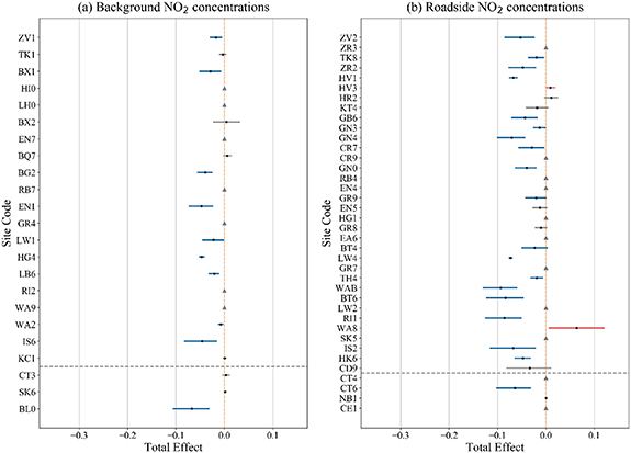
Figure 3. Estimated total effects on NO2 concentrations. Central estimates are indicated with black dots. The 95% CIs are illustrated with uncertainty bars (blue: pollution reduction; red: pollution increase). Null responses are denoted by grey triangles. A detected response that is statistically insignificant (at the 10% level) is indicated with grey interval bars. Sites within the ULEZ (below) and outside the ULEZ (above) are separated by the grey horizontal dashed line. Sites are sorted by the distance to the centroid of the ULEZ.
Download figure:
Standard image High-resolution imageTable 1. Summary of the ULEZ's effects on NO2 concentrations.
| Background NO2 | Roadside NO2 | ||||
|---|---|---|---|---|---|
| Total effect (%) ( a , b ) | Adj. R2 ( f ) | Total effect (%) ( a , b ) | Adj. R2 ( f ) | ||
| London | Response | 16 of 23 sites | 27 of 38 sites | ||
| std | 2.23 | 0.045 | 3.67 | 0.034 | |
| min | −6.75 | 0.870 | −9.34 | 0.877 | |
| max | 0.00 | 1.000 | 6.37 | 1.000 | |
| mean response ( c , e ) | −2.08*** [−3.44, −0.84] | −3.53*** [−5.11, −2.04] | |||
| regional mean( d , e ) | −1.44*** [−2.49, −0.49] | −2.53*** [−3.82, −1.35] | |||
| Within ULEZ | Response | 3 of 3 sites | 2 of 4 sites | ||
| std | 3.90 | 0.016 | 4.52 | 0.003 | |
| min | −6.75 | 0.969 | −6.40 | 0.995 | |
| max | 0.00 | 1.000 | 0.00 | 1.000 | |
| mean response ( c , e ) | −1.98 [−6.59, 0.61] | −3.14 [−8.67, 0.16] | |||
| regional mean( d , e ) | −1.98 [−6.59, 0.61] | −1.59 [−5.08, 0.07] | |||
| Outside ULEZ | Response | 13 of 20 sites | 25 of 34 sites | ||
| std | 1.91 | 0.048 | 3.71 | 0.034 | |
| min | −4.74 | 0.870 | −9.34 | 0.877 | |
| max | 0.00 | 1.000 | 6.37 | 1.000 | |
| mean response ( c , e ) | −2.08*** [−3.41, −0.81] | −3.54*** [−5.12, −1.91] | |||
| regional mean( d , e ) | −1.36*** [−2.37, −0.53] | −2.63*** [−3.87, −1.39] | |||
a The total effect includes the impact from the current period and the stacked impacts from the lagged periods. Interval estimate is simulated with 10 000 Monte Carlo iterations. Standard errors of coefficients are heteroscedasticity and autocorrelation consistent (HAC) using seven lags and without small sample correction. b The standard deviation, minimum value, and maximum value are provided with statistically insignificant estimates (at the 10% level) adjusted to zero. c The mean response is the aggregated effect across all sites where the concentrations responded to the intervention. d The regional mean is the aggregated effect across all sites. e The aggregated effect is computed with 1000 bootstrap resampling iterations. The 95% CI of aggregated effect (in bracket) is the percentile interval of 1000 bootstrap resampling iterations. Statistical significance: *** Significant at the 1% level; ** Significant at the 5% level; * Significant at the 10% level. f The adjusted R2 indicates the performance of the RDD model. The standard deviation, minimum value, and maximum value are provided by summarising the model performance across all RDD models.
The general response ratio of the monitoring sites within and outside the ULEZ are both similar to that at the city level. Within the ULEZ, NO2 concentrations were not statistically significantly reduced on average (regional mean) at either roadside (−1.98 [−6.59, 0.61]) or background stations (−1.59 [−5.08, 0.07]). Only one background site (BL0) and one roadside site (CT6) showed a significant decrease in NO2 concentrations while the others either showed insignificant or null responses. This implies that the decrease in traffic and the improvement in vehicle compliance rate was not sufficient to change the NO2 concentrations within the ULEZ.
Outside the ULEZ, the results at individual monitoring sites are heterogeneous: roadside NO2 concentrations experienced a greater response ratio (74%) and more negative mean response (−4%) than background concentrations (65%, −2%). However, we observe statistically significant pollution increases at two roadside sites (at a significance level of 10%), implying that the ULEZ increased road traffic emissions at some locations outside of the ULEZ.
For the sites that showed a significant change, the ULEZ reduced NO2 concentrations by <10%, as shown in figure 3. The highest reduction in background NO2 concentrations (7%) was at site BL0 within the ULEZ. The highest decrease in roadside NO2 concentrations (9%) was at site WAB outside the ULEZ.
The estimated effects of the ULEZ on NOx concentrations at different monitoring sites are illustrated in figure 4 and summarised in table 2. Further discussions of these results are provided in SI section S10. Comparing results for NOx with those of NO2, the London-level response ratio for NOx concentrations was smaller yet comparable for roadside sites (62% for NOx ; 71% for NO2), but much smaller for background sites (30% for NOx ; 70% for NO2). Considering the estimated effects at different monitoring sites, the NOx concentrations were more consistently decreased with a higher maximum reduction while an increase in NO2 concentrations was found at two roadside sites outside the ULEZ (at 10% significance level, cf figures 3 and 4).

Figure 4. Estimated total effects on NOx concentrations. Central estimates are indicated with black dots. The 95% CIs are illustrated with uncertainty bars (blue: pollution reduction; red: pollution increase). Null responses are denoted by grey triangles. A detected response that is statistically insignificant (at the 10% level) is indicated with grey interval bars. Sites within the ULEZ (below) and outside the ULEZ (above) are separated by the grey horizontal dashed line. Sites are sorted by the distance to the centroid of the ULEZ.
Download figure:
Standard image High-resolution imageTable 2. Summary of the ULEZ's effects on NOx concentrations.
| Background NOx | Roadside NOx | ||||
|---|---|---|---|---|---|
| Total effect (%) ( a , b ) | Adj. R2 ( f ) | Total effect (%) ( a , b ) | Adj. R2 ( f ) | ||
| London | Response | 7 of 23 sites | 24 of 39 sites | ||
| std | 3.83 | 0.105 | 2.96 | 0.035 | |
| min | −11.54 | 0.696 | −9.14 | 0.874 | |
| max | 0.00 | 1.000 | 0.99 | 1.000 | |
| mean response ( c , e ) | −3.83*** [−6.87, −1.56] | −4.22*** [−5.57, −2.87] | |||
| regional mean( d , e ) | −1.16*** [−2.38, −0.31] | −2.63*** [−3.77, −1.62] | |||
| Within ULEZ | Response | 1 of 3 sites | 2 of 4 sites | ||
| std | — | — | 4.51 | 0.002 | |
| min | −4.80 | 0.991 | −5.39 | 0.997 | |
| max | −4.80 | 0.991 | 0.99 | 1.000 | |
| mean response ( c , e ) | −4.80*** [−7.80, −2.02] ( g ) | −2.23 [−8.24, 1.74] | |||
| regional mean( d , e ) | −1.64 [−5.13, 0.00] | −1.14 [−4.68, 0.81] | |||
| Outside ULEZ | Response | 6 of 20 sites | 22 of 35 sites | ||
| std | 4.15 | 0.108 | 2.87 | 0.036 | |
| min | −11.54 | 0.696 | −9.14 | 0.874 | |
| max | 0.00 | 1.000 | 0.00 | 1.000 | |
| mean response ( c , e ) | −3.68*** [−7.36, −1.33] | −4.40*** [−5.89, −3.01] | |||
| regional mean( d , e ) | −1.09*** [−2.46, −0.16] | −2.79*** [−3.99, −1.65] | |||
a The total effect includes the impact from the current period and the stacked impacts from the lagged periods. Interval estimate is simulated with 10 000 Monte Carlo iterations. Standard errors of coefficients are HAC using seven lags and without small sample correction. b The standard deviation, minimum value, and maximum value are provided with statistically insignificant estimates (at the 10% level) adjusted to zero. c The mean response is the aggregated effect across all sites where the concentrations responded to the intervention. d The regional mean is the aggregated effect across all sites. e The aggregated effect is computed with 1000 bootstrap resampling iterations. The 95% CI of aggregated effect (in bracket) is the percentile interval of 1000 bootstrap resampling iterations. Statistical significance: *** Significant at the 1% level; ** Significant at the 5% level; * Significant at the 10% level. f The adjusted R2 indicates the performance of the RDD model. The standard deviation, minimum value, and maximum value are provided by summarising the model performance across all RDD models. g Only one site is in the group. In this case, the central estimate and 95% CI of the aggregated effect are represented by the corresponding metric of the effect estimate at this particular monitoring site.
The difference in response ratios for background NOx and NO2 concentrations likely reflects complex atmospheric chemical reactions involving NO, NO2, and O3. There are three monitoring sites that showed a significant increase (at the 10% level) in roadside concentrations of either NOx (site CT6) or NO2 (sites HV3 and WA8). However, since increases in both NOx and NO2 were not observed at any sites, the results imply that the change in concentrations of NOx and NO2 were highly site-specific and could have been influenced by atmospheric chemistry, vehicle flows, changes in vehicle fleet (i.e. ULEZ compliance) and changes in traffic speeds, which affect vehicle NOx emissions factors and the fraction of NOx emitted as NO2 (Clapp and Jenkin 2001, Carslaw 2005, O'Driscoll et al 2018, Carslaw et al 2019).
At kerbside sites, our results indicate that 71% and 43% of these showed a response to the ULEZ in NO2 and NOx concentrations respectively. Among the sites that showed a response, the ULEZ changed daily average kerbside NO2 concentrations by −13% to 0%, and NOx concentrations by −7% to −2%. The most significant pollution reductions were generally observed within the ULEZ or close to its boundary; however, some pollution reductions occurred at locations in outer London, implying that the ULEZ decreased road traffic emissions across a wider area. Compared with other types of monitoring sites, the kerbside sites had a similar response ratio to the roadside sites yet a higher maximum reduction (13% for kerbside; 9% for roadside) in NO2 concentrations. For NOx concentrations, the kerbside sites had a lower response ratio than roadside sites and all effect estimates for kerbside sites lie within the effect range for roadside and background sites (−12% to 1%).
Specifically, the highest reduction in kerbside NO2 concentrations (13%) was observed at the only site within the ULEZ; the highest reduction in kerbside NOx concentrations (7%) was at a site that is outside the zone yet next to its boundary. However, significant concurrent decreases in both NO2 and NOx concentrations were not observed at either of these sites. We also observe a diminishing improvement in air pollution at some locations. For example, at site WM6 within the ULEZ, the normalised concentrations of NO2 and NOx both started to increase in July 2019 after an initial reduction, and by September 2019, their levels reached a plateau where NOx had returned to the pre-ULEZ levels while NO2 remained lower than pre-ULEZ (see SI section S14). For NO2 and NOx , this 'rebound' also occurred for NO2 at a roadside site within the ULEZ, but not at any other roadside sites within the ULEZ nor kerbside sites close to the ULEZ.
The estimated effects of the ULEZ on PM10 concentrations at different monitoring sites are illustrated in figure 5. The consistent reduction in PM10 concentrations across monitoring sites due to ULEZ is counter-intuitive given that the regional contribution to the PM is substantial and the contribution of road traffic to PM10 concentrations is less than that for NOx (Greater London Authority 2020a). Our interpretation is that the results of PM10 can be attributed to seasonal and regional pollution transport effects rather than the ULEZ. Specifically, they could be related to the use of wood burning stoves and the growing contribution from this emissions sources in recent years. The use of wood accounted for 87% of PM emissions from domestic combustion in 2018, compared to 78% in 2008 (National Atmospheric Emissions Inventory 2021). In other words, there could be a year-on-year increase in this seasonality factor. As this increasing trend in the seasonality effect was not controlled for in the meteorological normalisation model, the PM10 concentration time series may not be fully normalised. An increase in daily average ambient temperature was observed in London after the start of the ULEZ (see SI section S9), therefore it is possible that the temperature change led to a decrease in domestic wood burning and consequently caused the observed reduction in PM10 concentrations.
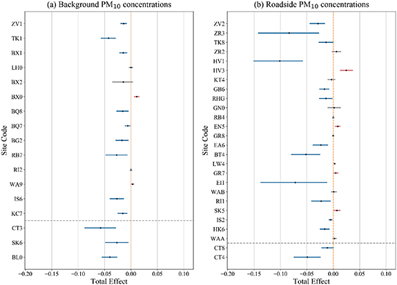
Figure 5. Estimated total effects on PM10 concentrations. Central estimates are indicated with black dots. The 95% CIs are illustrated with uncertainty bars (blue: pollution reduction; red: pollution increase). Null responses are denoted by grey triangles. A detected response that is statistically insignificant (at the 10% level) is indicated with grey interval bars. Sites within the ULEZ (below) and outside the ULEZ (above) are separated by the grey horizontal dashed line. Sites are sorted by the distance to the centroid of the ULEZ.
Download figure:
Standard image High-resolution imageThe estimated effects of the ULEZ on O3 and PM2.5 are summarised in table 3, which shows that the regional mean effect estimates across London were statistically insignificant at the 10% level. Results for these pollutants are discussed in detail in SI sections S8 and S9.
Table 3. Summary of the ULEZ's effects on O3 and PM2.5 concentrations.
| Background O3 | Roadside O3 | Background PM2.5 | Roadside PM2.5 | ||||||
|---|---|---|---|---|---|---|---|---|---|
| Total effect (%) ( a , b ) | Adj. R2 ( f ) | Total effect (%) ( a , b ) | Adj. R2 ( f ) | Total effect (%) ( a , b ) | Adj. R2 ( f ) | Total effect (%) ( a , b ) | Adj. R2 ( f ) | ||
| London | Response | 3 of 11 sites | 1 of 6 sites | 6 of 7 sites | 4 of 4 sites | ||||
| std | 2.70 | 0.056 | — | — | 1.45 | 0.062 | 3.00 | 0.035 | |
| min | −4.67 | 0.902 | 4.35 | 0.954 | 0.00 | 0.845 | −5.59 | 0.883 | |
| max | 0.00 | 1.000 | 4.35 | 0.954 | 3.56 | 1.000 | 0.94 | 0.958 | |
| mean response ( c , e ) | −1.71* [−4.23, 0.11] | 4.35** [0.81, 8.25]( g ) | 0.93 [−0.43, 2.60] | −1.70 [−5.14, 0.88] | |||||
| regional mean( d , e ) | −0.46 [−1.40, 0.02] | 0.74 [0.00, 2.92] | 0.79 [−0.31, 2.40] | −1.70 [−5.14, 0.88] | |||||
| Within ULEZ | Response | 0 of 2 sites | 0 site ( h ) | 1 of 2 sites | 0 site ( h ) | ||||
| std | — | — | — | — | — | — | — | — | |
| min | — | — | — | — | 0.35 | 1.000 | — | — | |
| max | — | — | — | — | 0.35 | 1.000 | — | — | |
| mean response ( c , e ) | — | — | 0.35** [0.01, 0.71]( g ) | — | |||||
| regional mean( d , e ) | 0.00 | — | 0.17 [0.00, 0.54] | — | |||||
| Outside ULEZ | Response | 3 of 9 sites | 1 of 6 sites | 5 of 5 sites | 4 of 4 sites | ||||
| std | 2.70 | 0.056 | — | — | 1.56 | 0.067 | 3.00 | 0.035 | |
| min | −4.67 | 0.902 | 4.35 | 0.954 | 0.00 | 0.845 | −5.59 | 0.883 | |
| max | 0.00 | 1.000 | 4.35 | 0.954 | 3.56 | 1.000 | 0.94 | 0.958 | |
| mean response ( c , e ) | 1.71* [−4.23, 0.11] | 4.35** [0.81, 8.25]( g ) | 1.03 [−0.67, 2.97] | −1.70 [−5.14, 0.88] | |||||
| regional mean( d , e ) | −0.56 [−1.64, 0.03] | 0.74 [0.00, 2.92] | 1.03 [−0.67, 2.97] | −1.70 [−5.14, 0.88] | |||||
a The total effect includes the impact from the current period and the stacked impacts from the lagged periods. Interval estimate is simulated with 10 000 Monte Carlo iterations. Standard errors of coefficients are HAC using seven lags and without small sample correction. b The standard deviation, minimum value, and maximum value are provided with statistically insignificant estimates (at the 10% level) adjusted to zero. c The mean response is the aggregated effect across all sites where the concentrations responded to the intervention. d The regional mean is the aggregated effect across all sites. e The aggregated effect is computed with 1000 bootstrap resampling iterations. The 95% CI of aggregated effect (in bracket) is the percentile interval of 1000 bootstrap resampling iterations. Statistical significance: *** Significant at the 1% level; ** Significant at the 5% level; * Significant at the 10% level. f The adjusted R2 indicates the performance of the RDD model. The standard deviation, minimum value, and maximum value are provided by summarising the model performance across all RDD models. g Only one site is in the group. In this case, the central estimate and 95% CI of the aggregated effect are represented by the corresponding metric of the effect estimate at this particular monitoring site. h No sites in the region met the data quality criteria.
3.3. ULEZ effects in the context of long-term trends
The introduction of the ULEZ is only one of several air pollution mitigation policies that have been undertaken in London in recent years; other policies include the LEZ, Low Emission Bus Zones, bus retrofit, Taxi Delicensing Scheme, zero emission capable requirement on new taxis, and Euro vehicle emissions standards (Greater London Authority 2020a). A trend analysis on normalised air pollutant concentrations at individual monitoring sites shows a general trend in London's air quality levels since 2016 across various locations; generally decreasing for NO2, NOx , and PM concentrations, and increasing for O3 concentrations (figure 6). It is noted that the increasing trend in O3 concentrations can be related to the decrease in NOx concentrations; in cities, a decrease in NOx concentrations typically leads to an increase in O3 concentrations due to the chemical coupling of these pollutants (Clapp and Jenkin 2001, Diaz et al 2020). Additionally, comparing the trend in different years, the most rapid pollution reductions generally occurred before the launch of the ULEZ (figure 7). Taken along with our main results, this implies that it is the combined effects of several policies that have led to improvements in air quality (for NO2, NOx , and PM), and that the ULEZ on its own is unlikely to be the most significant contributor to air pollution reduction in recent years.
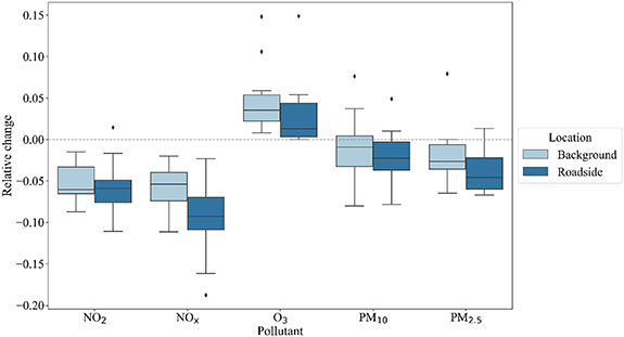
Figure 6. Rate of change in concentrations of different air pollutants in London in recent years. Trends at individual monitoring sites are estimated on normalised air pollutant concentrations from 2016-01-01 to 2020-01-31, where the influences of meteorological conditions and seasonality effects are removed. Relative changes at individual monitoring sites are derived by normalising the trend estimate with the corresponding annual average concentration in 2016. The boxplot is provided with the statistically insignificant trend estimates (at the 10% level) adjusted to zero.
Download figure:
Standard image High-resolution image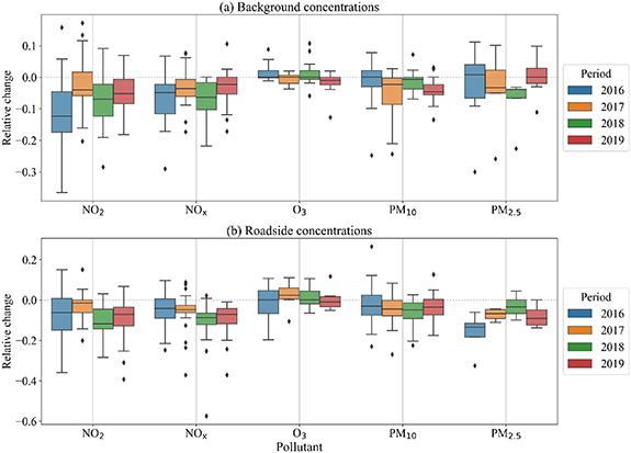
Figure 7. Rate of change in air pollution in London in different years from 2016 to 2019. Trends are estimated on normalised air pollutant concentrations at individual monitoring sites, separately for each year from 2016 to 2019. Air pollutant concentrations are normalised to remove the influences of meteorological conditions and seasonality effects. Relative changes are derived by normalising the trend estimates with the annual average concentration at individual monitoring sites in a specific year. The boxplot is provided with the statistically insignificant trend estimates (at the 10% level) adjusted to zero.
Download figure:
Standard image High-resolution image
4. Conclusions
This paper provides an ex-post causal analysis of the effectiveness of the London ULEZ on improving air quality at different pollution monitoring sites. Our estimates show that the ULEZ was effective in the sense that it caused changes in air pollution at various locations within 5–8 weeks around the introduction; 70% (71%), 50% (49%), and 24% (28%) of the monitoring sites (percentages in brackets include kerbside sites) showed a response to the ULEZ for NO2, NOx , and O3 concentrations, respectively. For those sites where a response was detected, the majority of effect estimates indicated a reduction in air pollution, yet some increases were observed. Effect estimates at roadside and background sites ranged from −9% to 6% for NO2, −12% to 1% for NOx , −5% to 4% for O3, and −6% to 4% for PM2.5. Aggregating the effects at roadside and background monitoring sites, the mean effects across London were small; up to 3% reduction for NO2 and NOx , and insignificant for O3 and PM2.5. NO2 concentrations at locations within the ULEZ more consistently decreased, while a small increase (within 6%) in air pollution were found at two roadside monitoring sites outside the ULEZ. These results imply that the ULEZ on its own was not effective in the sense that the marginal effects caused by the ULEZ on improving air quality were small, either at particular locations or averaging across London. Air quality (for NO2, NOx , and PM) has improved in London in recent years and the most significant pollution reductions were generally found before 2019. This indicates that reducing air pollution requires a multi-faceted set of policies that aim to reduce emissions across sectors with coordination in the city, regional, and transboundary scales. Meanwhile, it is likely that the ineffectiveness of Euro standards has also diminished the ULEZ's potential effect: while the regulatory limit for NOx emissions decreased by 56% between Euro 5 and Euro 6, the evidence from real-world emissions testing indicates that this reduction has not been fully realised and that emissions of Euro 6 vehicles are several times higher than the regulatory standard (O'Driscoll et al 2016, 2018).
Compared with analyses by the Greater London Authority, our results indicate that a smaller reduction in air pollution can be attributed to the ULEZ. The Greater London Authority (2019, 2020b) attributed a 29% reduction in roadside NO2 concentrations in central London from July to September 2019 and a 37% reduction from January to February 2020 to the ULEZ. This is higher than our effect estimates both at the monitoring site level and at the regional level. The data sources and the research period after the introduction of the ULEZ of these analyses are similar to our study. The differences in estimates are due to the methodological choice and the research period specification. The Greater London Authority (2019, 2020b) estimated the causal effects of the ULEZ following the DID approach, using the situation in outer London as a control group and the period before the T-charge announcement as the pre-intervention period. By comparing the situations before the T-charge and after the ULEZ, the effect estimate is a combined effect of these two policies and it is therefore unsurprising that it is higher than the effect of the ULEZ alone, as with our estimates. Furthermore, effect estimates based on comparing these two periods could be biased without control for seasonality effects. As for using the situation in outer London as a control group, it is necessary to assume that the air quality in central London would have followed the same trend as in outer London in absence of the ULEZ and we note that the factors affecting pollutant emissions (such as demographics, car ownership, and composition of the vehicle fleet) are different in these two areas, and some interventions have been prioritised (such as the bus fleet upgrade) or only implemented (such as the removal of PHV exemption) in central London.
In this paper, we follow the methodology in Ma et al (2021) with further improvements in the CPD and causal inference processes. However, we note that the method is subject to some limitations that should be further explored, such as the attribution of the estimated effect to different industrial sectors, the bias potentially from omitted important baseline covariate(s), and the separation of effects when another intervention was simultaneously implemented. Future work should investigate asymmetric donut holes, the relationship between the margin period and donut hole, and meteorological normalisation techniques that can control for the evolution of seasonality effects and incorporate factors to account for regional pollution import (such as regional meteorological conditions and air pollution levels at source regions), which affect PM concentrations in particular.
Acknowledgments
L M is funded by the Dixon and Skempton Scholarships from the Department of Civil and Environmental Engineering, Imperial College London. Certain images in this publication have been obtained by the author(s) from the Wikipedia/Wikimedia website, where they were made available under a Creative Commons licence or stated to be in the public domain. Please see individual figure captions in this publication for details. To the extent that the law allows, IOP Publishing disclaim any liability that any person may suffer as a result of accessing, using or forwarding the image(s). Any reuse rights should be checked and permission should be sought if necessary from Wikipedia/Wikimedia and/or the copyright owner (as appropriate) before using or forwarding the image(s).
Data availability statement
The data that support the findings of this study are available upon reasonable request from the authors.