

Abstract
Understanding future changes in global terrestrial near-surface wind speed (NSWS) in specific global warming level (GWL) is crucial for climate change adaption. Previous studies have projected the NSWS changes; however, the changes of NSWS with different GWLs have yet to be studied. In this paper, we employ the Max Planck Institute Earth System Model large ensembles to evaluate the contributions of different GWLs to the NSWS changes. The results show that the NSWS decreases over the Northern Hemisphere (NH) mid-to-high latitudes and increases over the Southern Hemisphere (SH) as the GWL increases by 1.5 °C–4.0 °C relative to the preindustrial period, and that these characteristics are more significant with the stronger GWL. The probability density of the NSWS shifts toward weak winds over NH and strong winds over SH between the current climate and the 4.0 °C GWL. Compared to 1.5 °C GWL, the NSWS decreases −0.066 m s−1 over NH and increases +0.065 m s−1 over SH with 4.0 °C GWL, especially for East Asia and South America, the decrease and increase are most significant, which reach −0.21 and +0.093 m s−1, respectively. Changes in the temperature gradient induced by global warming could be the primary factor causing the interhemispheric asymmetry of future NSWS changes. Intensified global warming induces the reduction in Hadley, Ferrell, and Polar cells over NH and the strengthening of the Hadley cell over SH could be another determinant of asymmetry changes in NSWS between two hemispheres.
Export citation and abstract BibTeX RIS

Original content from this work may be used under the terms of the Creative Commons Attribution 4.0 license. Any further distribution of this work must maintain attribution to the author(s) and the title of the work, journal citation and DOI.
1. Introduction
Terrestrial near-surface wind speed (NSWS) is a key parameter of atmospheric circulation and climate change. Investigating NSWS dynamics can provide theoretical insights for evaluations of wind energy (Zhang et al 2019a, Pryor et al 2020), regional evapotranspiration (McVicar et al 2012), hydrological cycles (Liu et al 2014), air pollution (Zhang et al 2020), and dust storms (Wang et al 2017), among other socioeconomic and environmental implications. As the climate warmed in the last several decades, the global terrestrial NSWS exhibited a decrease (Wu et al 2018a). Roderick et al (2007) termed the general reduction in NSWS 'stilling'. The terrestrial stilling is also observed at regional-scale (Azorin-Molina et al 2014, Wu et al 2016, Gilliland and Keim 2018, Zhang and Wang 2020). In contrast to the terrestrial stilling, an increase in NSWS that's been reported globally since 2010 (Zeng et al 2019), and Zeng et al (2019) termed the general increase in NSWS 'reversal'. An increase in regional NSWS is also observed in recent decades (Kim and Paik 2015, Li et al 2018, Zha et al 2021a).
Except for the investigations of historical NSWS changes, the future NSWS changes are also studied based on the multi-model ensemble (MME) of Coupled Model Intercomparison Project Phase 5/6 (CMIP5/6) in the current studies. Kumar et al (2015) analyzed the changes of wind extremes and proposed a decline in the magnitude of extreme NSWS over Northern Hemisphere (NH). Karnauskas et al (2018) revealed wind power decreased over the NH mid-latitudes and increased over the tropics and the Southern Hemisphere (SH) under representative concentration pathway (RCP) 4.5 (RCP4.5) and 8.5 (RCP8.5). Goyal et al (2021) discovered a projected end of 21st century SH surface westerlies increased of ∼10% and a poleward shift of ∼0.8° latitude based on MME of CMIP5. Some studies have found that the greenhouse-gas (GHG)-induced global warming contributed to the slowdown in NSWS (Bichet et al 2012, Gao et al 2018, Zha et al 2020, Shen et al 2021b). The significance of GHG to the changes of NSWS is also demonstrated based on CMIP5 (Jiang et al 2010, Chen et al 2012). Global warming can cause the changes in ocean–atmosphere oscillation, and therefore, Zeng et al (2019) highlighted the role of ocean–atmosphere oscillation in explaining stilling and reversal phenomena.
Internal variability in the climate system complicates the estimation of human-induced climate change and imposes irreducible limits on the accuracy of climate projections (Deser et al 2020). Consequently, the effects of human-induced warming on future NSWS changes are predicted with large uncertainty if the basis is only a global climate model or MME, due to internal variability cannot be well excluded (Torralba et al 2017, IPCC 2021). Moreover, the MME of CMIP5/6 may underestimate the magnitude of warming, and therefore, affect the accuracy of results (Li et al 2019). The large ensembles (LEs) allow us to extract the effects of external forcing (e.g. GHG-induced global warming), due to the internal variability of models can be eliminated based on the ensemble mean of LEs. The model bias can also be partly removed when using integrations of individual LEs to compute climate trends (Yu et al 2020).
Although Karnauskas et al (2018) has projected the changes of global NSWS based on ten CMIP5 models, the contribution of specific global warming level (GWL) to NSWS changes is not discussed and the influences of internal variability on NSWS are not excluded. To our knowledge, no study focused on the contributions of specific GWL to the NSWS changes. To what extent the wind change is influenced by specific GWL and whether the interhemispheric asymmetry of future NSWS will change with different GWLs are important issues, and which should be investigated. In this study, accompanied by the removal of internal variability, the influences of different GWLs on NSWS changes are projected and the causes of the intensified GWL affects NSWS are analyzed. This study provides a reference for improving our understanding of NSWS changes. Meanwhile, it also provides a scientific basis for decision-makers to formulate policies to deal with climate change.
2. Datasets and methods
2.1. Datasets
The Max Planck Institute Earth System Model (MPI-ESM) is used in this study, which is the largest ensemble (100-member ensemble of simulations) of a single state-of-the-art comprehensive climate model currently available (https://esgf-data.dkrz.de/projects/mpi-ge/, last accessed on 25 June 2021). The performance of MPI-ESM LEs has been evaluated (Reichler et al 2012, Charlton-Perez et al 2013), and which has been extensively used to understand the effects of internal variability and external forcing (Maher et al 2018). The MPI-ESM is a fully coupled atmosphere–ocean model with a horizontal resolution of 1.9° × 1.9° and 47 vertical layers up to 0.01 hPa (Reick et al 2013). Individual members of the MPI-ESM only differ in their initial conditions (Bittner et al 2016), and the initialization branching time for each member from the preindustrial control run is introduced in Maher et al (2019). The historical simulations are integrated from 1850 to 2005, driven by observed radiative forcing. Future projections, not forecasts, are taken considering the most pessimistic future GHG emission rates, the RCP8.5 scenario, which represents that GHG emissions will lead to 8.5 W m−2 radiative forcing (Costoya et al 2020). Furthermore, the strong warming magnitude cannot be reached with low emission scenario. Therefore, the future simulation from 2006 to 2099 with the RCP8.5 is used in this study (Monerie et al 2017, Huang et al 2020). In MPI-ESM, the land component is the JSBACH model including dynamic vegetation and land use transitions with the standard fire module (Maher et al 2019). The land use and cover change is considered in MPI-ESM LEs, and which includes the natural and anthropogenic land cover change (Reick et al 2013). The natural land cover change features two types of competition: between the classes of grasses and woody types controlled by disturbances (fire and windthrow) and within those vegetation classes between different plant functional types based on relative net primary productivity advantages (Reick et al 2013). The anthropogenic land cover change implements the land use transition approach by Hurtt et al (2006).
Three global reanalysis datasets are used to estimate the performance of MPI-ESM in simulating the NSWS. (a) The European Centre for Medium-Range Weather Forecasts fifth generation of atmospheric reanalysis (ERA5), (b) the National Centers for Environmental Prediction and National Center for Atmospheric Research reanalysis-1 (NCEP1), and (c) the Japanese 55 year reanalysis from Japan Meteorological Agency (JRA55) (table S1 available online at stacks.iop.org/ERL/16/114016/mmedia). These datasets hanvestigate the NSWS changes at global-scale (Ramon et al 2019, Fan et al 2021). In this study, monthly mean values of the MPI-ESM LEs and the reanalysis datasets are used.
To examine whether the MPI-ESM can simulate the terrestrial stilling, Global Surface Summary of the Day (GSOD) database is used (available at ftp://ftp.ncdc.noaa.gov/pub/data/gsod, last accessed on 25 June 2021). GSOD database consists of the United States Air Force DATSAV3 surface dataset and the Federal Climate Complex Integrated Surface Hourly dataset (Funk et al 2015). To obtain a high-quality wind record, Zeng et al (2019) have employed strict section criteria to avoid incomplete data series, and they concluded that the NSWS data at 1435 stations provide the most useful information. We utilize the data from those same 1435 stations in this study. The stations mainly locate in NH, so we compare the observation with MPI-ESM across NH to evaluate the performance of MPI-ESM in simulating the stilling.
2.2. Methods
The observed global mean near-surface air temperature (GMST) is about 1 °C warming relative to the preindustrial period; therefore, we define the 1.0 °C warming period in 1995–2004 in MPI-ESM as the current climate (baseline period). As such, the GMST increased by 1.5 °C, 2 °C, 3 °C, 4 °C compared with the preindustrial level in the models corresponding to the following four 10 year periods in MPI-ESM: 2015–2024 (1.50 °C), 2031–2040 (2.00 °C), 2055–2064 (2.99 °C), and 2077–2086 (4.02 °C). The GMST and NSWS changes are analyzed relative to the current climate. The GMST in the recent 30 year (1986–2015) increased by approximately 0.69 °C above the preindustrial level. To maintain the GMST increased by the same amount (0.69 °C), the model-simulated 30 year (1971–2000) mean values of NSWS in MPI-ESM LEs are compared with three reanalysis datasets (ERA5, NCEP1, and JRA55) during the period (1986–2015) when the GMST increased by the same amount (∼0.69 °C) above the preindustrial level.
To understand the causes of NSWS changes under different GWLs, the meridional temperature gradient (MTG) is calculated. Four latitude zones are defined: LZ1 (60° N to 90° N; 180° W to 180° E), LZ2 (0° to 60° N; 180° W to 180° E), LZ3 (45° S to 90° S; 180° W to 180° E), and LZ4 (0° to 45° S; 180° W to 180° E). The MTG is calculated using equation (1)
The trend is calculated using the least-square method, and the significance of the result is tested using the two-tailed Student's t-test. Reviewing previous studies (Chevuturi et al 2018, Cannon 2020), the globe is divided into eight regions: North America (25° N–72° N, 170° W–50° W), South America (60° S–20° N, 80° W–30° W), Europe (30° W–45° E, 30° N–75° N), Central Asia (30° N–65° N, 45° E–100° E), South Asia (5° N–35° N, 65° E–100° E), East Asia (10° N–79° N, 100° E–150° E), Africa (50° S–10° S, 110° E–160° E), and Australia (40° S–20° N, 20° W–55° E) (figure 1(a)).
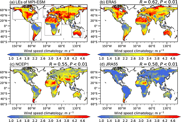
Figure 1. Spatial patterns of global mean terrestrial near-surface wind speed in (a) MPI-ESM LEs, (b) ERA5, (c) NCEP1, and (d) JRA55 during the period when global mean near-surface temperature increases by the same amount above the preindustrial level. R denotes the spatial correlation coefficient, and P < 0.01 is used as the threshold for statistical significance. In (a), the defined regions are shown as North America (region 1), Europe (region 2), Central Asia (region 3), East Asia (region 4), South America (region 5), Africa (region 6), South Asia (region 7), and Australia (region 8).
Download figure:
Standard image High-resolution image3. Results
3.1. Verification of MPI-ESM in simulating the NSWS
Spatial patterns of NSWS in MPI-ESM and reanalysis datasets are compared (figure 1). The large values of NSWS (>4.0 m s−1) mainly locate in North America, Northern Africa, Asia, and Australia, and the small values of NSWS (<2.0 m s−1) mainly locate in South America and Southern Africa (figure 1(a)). A similar spatial pattern of NSWS climatology is well reproduced in ERA5 (figure 1(b)) and NCEP1 (figure 1(c)). The wind speed difference between MPI-ESM and ERA5 is between ±1.0 m s−1 in most regions of globe (figure S1(a)), and the MPI-ESM and NCEP1 mainly show positive bias but for the regions between 20° N and 20° S (figure S1(b)). Previous study has revealed that the NSWS climatology in ERA5 is closest to the observation due to the high spatiotemporal resolution in ERA5 compared to other reanalysis datasets (Fan et al 2021). This result indirectly demonstrate that the MPI-ESM LEs can capture the observed NSWS climatology. The mean NSWS in JRA55 is smaller than that in others (figure 1(d)), and the wind speed difference between MPI-ESM LEs and JRA55 exhibits positive value across globe (figure S1(c)). Previous studies have illustrated that the negative NSWS bias in JRA55 generates from the lowermost atmospheric level, which is placed too high over regions with trees, thus reducing the wind speed when interpolated from that level down to the altitude of 10 m, and are not fully corrected in the data assimilation process (Torralba et al 2017, Zhang et al 2020). Furthermore, JRA55 has a coarse resolution. These could explain why JRA55 has smaller NSWS compared to other reanalysis datasets.
Temporal changes of the NSWS in three reanalysis datasets mainly locate in the inter-model spreads of LEs, although the interannual changes in NSWS are not consistent (figure S2(a)). It is generally believed that the LEs can capture the climatology and dynamics of variables if the temporal series of reanalysis products can be included in the inter-model spreads of LEs (Li et al 2019). A significant decrease in NSWS is found in JRA55 (−0.021 m s−1 decade−1; p< 0.05), and this could be because the observed NSWS is assimilated in JRA55. According to our knowledge, only JRA55 assimilate observed NSWS over land into the reanalysis, but other reanalysis products assimilate winds over ocean (Fujiwara et al 2017, Torralba et al 2017, Zhang and Wang 2020). JRA55 simulates the long-term trend of NSWS could be better than other reanalysis products, but which shows largest absolute deviation of NSWS. Hence, it cannot be said that JRA55 simulates the global NSWS is better or worse than other reanalysis products. To confirm whether the stilling can be observed in LEs, the ensemble mean of members with negative trends in MPI-ESM is compared with the observation over the NH (figure S2(b)). The stilling can be observed in MPI-ESM LEs, although the stilling in MPI-ESM (−0.03 m s−1 decade−1; p< 0.01) is weaker than observation (−0.08 m s−1 decade−1; p< 0.01). In this study, we focus on the effects of the specific GWL on the long-term changes in NSWS when the effects of internal variability are excluded. The magnitude of trend in ensemble mean NSWS in MPI-ESM is smaller than observation, which is likely because the effects of internal variability are counteracted and the interannual fluctuations of NSWS are smoothed when the ensemble mean is carried out (Deser et al 2012, Wu et al 2018b, Shen et al 2021a).
3.2. Future changes in NSWS with different GWLs
Figure 2 shows the spatial patterns of annual mean NSWS changes with different GWLs. As the GMST increases by 1.5 °C–4 °C, the NSWS decreases over the NH mid-to-high latitudes and increases over the SH (except for Australia). The reduction in NSWS is more significant over North America and Eurasia and the increase is more pronounced over South America and Southern Africa. Relative to the current climate, under 1.5 °C, 2 °C, 3 °C, and 4 °C GWLs, the NSWS decreases by −0.015 ± 0.003, −0.016 ± 0.004, −0.029 ± 0.003, and −0.045 ± 0.004 m s−1 over the globe, respectively; it decreases (increases) by −0.030 ± 0.0023 (+0.023 ± 0.005), −0.041 ± 0.005 (+0.052 ± 0.005), −0.070 ± 0.003 (+0.078 ± 0.005), and −0.095 ± 0.005 (+0.089 ± 0.007) m s−1 over the NH (SH), respectively. With the same GWL, a substantial decrease in NSWS is detected in Asia and, with the strongest decrease occurs in South Asia (figure 3). Additionally, a substantial increase occurs in South America, especially for the 4 °C GWL where the future NSWS increases by +0.130 ± 0.010 m s−1 relative to the current climate (figure 3). Consequently, the projected asymmetry changes in NSWS between two hemispheres could strengthen with the intensified GWL. Similar to the annual mean NSWS, the seasonal NSWSs also mainly decrease over the NH mid-to-high latitudes and increase over the SH; however, the seasonal NSWSs do not exhibit the decreasing trend over most regions of East Asia with the low GWL (e.g. 1.5 °C GWL) (figure S3). The temporal changes of the seasonal NSWS can also reveal the interhemispheric asymmetry of NSWS changes, although the seasonal differences of NSWS are evident and the interannual variations of NSWS are different among seasons (figure S4).
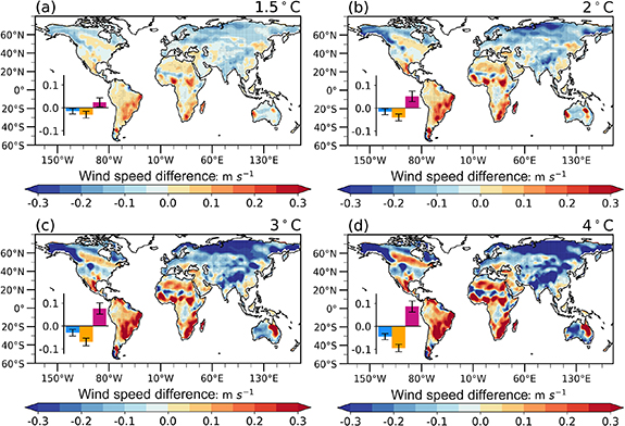
Figure 2. Spatial patterns of changes (relative to the current climate) in global terrestrial near-surface wind speed when global mean near-surface temperature increases by 1.5 °C–4 °C above the preindustrial level. (a)–(d) pertain to 1.5 °C, 2 °C, 3 °C, and 4 °C global warming level, respectively. Dots denote where the wind speed difference is statistically significant at the 0.10 level. In the insets, the blue, yellow, and red histograms denote the mean values of the wind speed difference over the globe, Northern Hemisphere, and Southern Hemisphere, respectively. The black error bars denote the uncertainties of the results, which are calculated based on the 100 members of large ensembles in MPI-ESM.
Download figure:
Standard image High-resolution image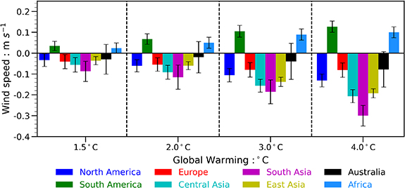
Figure 3. Changes (relative to the current climate) in near-surface wind speed over the main regions of the globe when global mean near-surface temperature increases by 1.5 °C–4 °C above the preindustrial level. The black error bars denote the uncertainties of the results, which are calculated based on the 100 members of large ensembles in MPI-ESM.
Download figure:
Standard image High-resolution imageFigure 4 shows scatter plots between the NSWS and GMST changes. There is a linear relationship between the global NSWS decreases and GMST increases. The correlation coefficient is −0.91 (p< 0.01) (figure 4(a)). The NSWS and GMST are also negatively related over the NH (−0.98, p< 0.01). In contrast, these variables are positively related over the SH (0.94, p< 0.01). With 1.5 °C–2 °C (0.5 °C), 1.5 °C–3 °C (1.5 °C), and 1.5 °C–4 °C (2.5 °C) warming, the NSWS decreases −0.012 ± 0.004, −0.040 ± 0.004, and −0.066 ± 0.004 m s−1 over the NH, respectively (figure 4(b)), and which increases +0.029 ± 0.006, +0.048 ± 0.004, and +0.069 ± 0.004 m s−1 over the SH, respectively (figure 4(c)). The NSWS and GMST changes also exhibit negative correlations in most regions of NH and positive correlations in South America and Africa of SH (figure S5). These results confirm that decreases in global NSWS attribute to the intensified global warming occur mainly in the NH; whilst the NSWS over the SH could increase. There is low confidence in projected mean wind speed over Australia, with a medium confidence increase projected in northeastern Australia under high emission scenarios by the end of the 21st century (IPCC 2021). The monsoon is one of the most important climatic phenomena on Earth that can influence the wind changes (An et al 2015). The differential heating between land and ocean induced by monsoon causes the temperature gradient changes, and the latter can induce the changes in pressure gradient that is the driving force of wind speed changes (Wu et al 2018a). Noting that the projected Australian monsoon shows large uncertainty (IPCC 2021); therefore low confidence in projected NSWS changes over Australia may be linked to the large uncertainty in projected monsoon circulation changes.
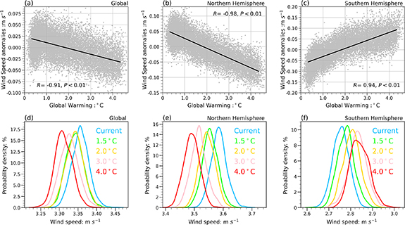
Figure 4. (a)–(c) Relationships between the averaged near-surface wind speed (NSWS) anomaly (m s−1) and global warming level (°C), and (d)–(f) probability density functions (PDFs) of changes (relative to the current climate) in NSWS (%) under different global warming levels. In (a)–(c), gray dot presents the NSWS and GMST at each members in each year, which reflects the changes in the NSWS and global mean near-surface temperature (GMST) relative to the current climate (1995–2004), and the solid black lines denote the linear fitting curves. R denotes the correlation coefficient, and p < 0.01 is used as the threshold for statistical significance. In (d)–(f), blue, green, yellow, light red, and red solid lines represent histograms of the current climate and a GMST increase of 1.5 °C, 2 °C, 3 °C, and 4 °C above the preindustrial level, respectively.
Download figure:
Standard image High-resolution imageProbability density functions (PDFs) of NSWS under different GWLs are investigated (figures 4(d)–(f)). The NSWS PDFs clearly shift leftward but with little change in shape between the current climate and 4.0 °C warming, indicating a reduction in NSWS mean value but not the variability in NSWS (figure 4(d)). In terms of the NH, the NSWS PDFs also shift leftward but with little change in shape between the current climate and 4.0 °C warming; nevertheless, the NSWS over the NH is larger than global NSWS (figure 4(e)). With respect to SH, the NSWS PDFs shift rightward and the maximum probability density of NSWS reduces with the strengthened global warming, indicating an increase in NSWS mean value over the SH (figure 4(f)). Regional characteristics of NSWS PDFs show that the enhanced global warming causes the NSWS PDFs to move toward weak wind over North America, Europe, and Asia, especially for Central Asia, East Asia and South Asia, this characteristic is more pronounced. Nevertheless, the NSWS PDFs show opposite changes over South America and Africa, indicating that the intensified global warming is beneficial to the increase in NSWS over these two regions (figure S6).
3.3. Potential causes of interhemispheric asymmetry of NSWS changes
It is acknowledged that the global warming is more pronounced over high latitudes than that over low latitudes (IPCC 2021). In this study, we also confirm that the increase in GMST is more significant over the NH mid-to-high latitudes than that in other regions under different GWLs based on MPI-ESM LEs (figure S7). It is worth noting that the increase in GMST over the SH, especially for the regions between 45 and 80° S, is less than 1.0 °C even where strong global warming occurs (figures S7(c) and (d)).
Temperature gradient is the primary driving force of NSWS (Wu et al 2018a). Global warming could induce the changes in temperature gradient (You et al 2010). To understand how enhanced warming influences the NSWS changes, the MTG is calculated. The MTG decreases over the NH and increases over the SH, at rates of −0.027 and +0.210 °C decade−1, respectively, and that these characteristics are reproduced in the inter-model spreads of 100 members (figures 5(a) and (b)). The MTG and NSWS anomaly show positive correlation, with correlation coefficients of 0.88 (p< 0.01) over NH and 0.96 (p< 0.01) over SH (figure 5(c) and (d)). Quantitatively, each 0.5 °C decrease (rise) in MTG over NH (SH) causes a −0.20 ± 0.018 m s−1 (+0.28 ± 0.001 m s−1) decrease (increase) in NSWS over NH (SH). Briefly, the MTG decreases in NH and increases in SH attributes to unevenly global warming may be responsible for the NSWS decreases in NH and increases in SH.
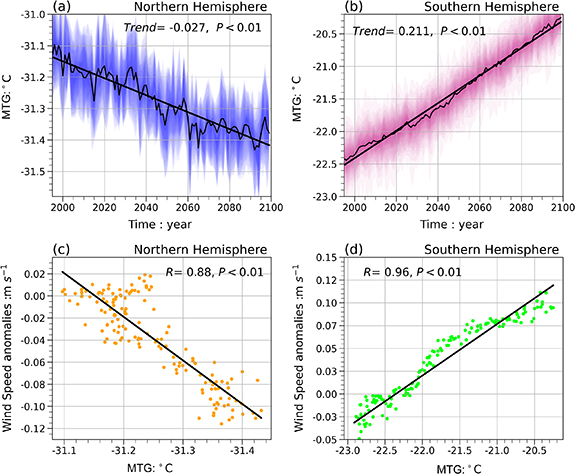
Figure 5. Temporal changes in the meridional temperature gradient (MTG) over the (a) Northern Hemisphere and (b) Southern Hemisphere between 1995–2099 (°C), as well as a regression analysis between MTG and near-surface wind speed anomaly over the (c) Northern Hemisphere and (d) Southern Hemisphere. In (a), (b), the shading denotes the inter-model spreads of 100 members in MPI-ESM LEs. Black lines denote the linear fitting. Trend is the linear trend, which is calculated based on the least-square method. R is the correlation coefficient, and p < 0.01 is used as the threshold for statistical significance.
Download figure:
Standard image High-resolution imageChanges in vertical atmospheric circulation could affect NSWS changes, so we detect the effects of different GWLs on the vertical atmospheric circulation. Three cells (Hadley, Ferrell, and Polar cells) are fairly reproduced with four GWLs (figure S8). However, with the enhancement of global warming, ascending flows are detected between 20 and 30° N and between 70 and 90° N, and descending flows are detected between 40 and 60° N (figure 6). Compared to the climatology of vertical atmospheric circulation (figure S8), the Hadley, Ferrell, and Polar cells are restrained due to the opposite vertical motions occur in the regions of descending flows in the Hadley cell and polar cell, and ascending flows in the Ferrell cell; as well as the inhibiting effects are more pronounced with the stronger GWL. Consequently, the strengthening in global warming may cause the weakening of the three cells over NH, and the latter result in a reduction in NSWS over NH. In SH, with the enhancement of global warming, descending flows are detected between 30 and 52° S and ascending flows are detected between 52 and 67° S. Consequently, the descending flows between 30 and 52° S triggered by strong GWL heighten the descending flows of the Hadley cell over the SH, while the location of descending flows in the Hadley cell moves slightly southward (Hu and Fu 2007). Consequently, the strengthened Hadley cell strengthens in SH due to the strengthening of global warming could induce the increase in NSWS over SH. Actually, these vertical cells influence historical wind speed changes have been discussed in the previous studies (Hu and Fu 2007, Deng et al 2021, Shen et al 2021a).

Figure 6. Vertical structures of changes (relative to the current climate) in zonal-mean vertical velocity (shading: 10−3 Pa s−1) and zonal-mean vertical wind (vector: m s−1) when global mean near-surface temperature increases by 1.5 °C–4 °C above the preindustrial level. The vector is that of wind speed difference, whose two components are the zonal-mean meridional wind speed difference and the zonal-mean vertical velocity difference between different global warming levels and current climate. The purple arrows denote the ascending flows and green arrows denote the descending flows. Shading and vectors denote significance at the 0.10 level.
Download figure:
Standard image High-resolution image
4. Discussions
Previous studies have shown that the observed NSWS in the NH has experienced a significant reduction on decadal scale (Vautard et al 2010, Tian et al 2019, Zhang et al 2019b), although a slight increase has been reported in the recent decade (Zeng et al 2019). Based on CMIP6, Deng et al (2021) found that the historical NSWS experienced a decrease over the NH and an increase over the SH in the past several decades, and proposed that atmospheric circulation changes attributed to high emission had an effect on historical NSWS. Our results further confirm that the intensified global warming may contribute to a reduction in NSWS over the NH and an increase over the SH (except for Australia) in the future. Therefore, the present reversal of stilling over the NH may only be a short-term phenomenon before winds start decreasing again if the global warming cannot be controlled effectively. However, to improve the significance of the results and better satisfy the necessity of the decision-makers, a fully coupled equilibrium climate simulations are necessary. We should produce a set of scenarios using multi-model designed to achieve long-term different GWLs in a stable climate, and employ these scenarios to implement century-scale ensemble simulations (Sanderson et al 2017). Meanwhile, evaluating the significance of impact differences with respect to multi-model variability.
We propose that the changes in MTG and three cells induced by global warming could influence the NSWS changes. Nevertheless, the MTG and three cells can also cause the changes in large-scale ocean-atmosphere circulations (LOACs). Several studies have discussed the effects of LOACs on wind changes (Timmermann et al 2018, Zhang et al 2018). Zeng et al (2019) suggested that the NSWS changes in NH could be attributed to Tropical Northern Atlantic, North Atlantic Oscillation, and Pacific Decadal Oscillation. However, the interaction and modulation among different LOACs are complicated, and therefore, the NSWS changes should be determined by the combined effects of variations in multiple LOACs (Shen et al 2021a, Zha et al 2021a). Hence, the mechanisms whereby LOACs affect NSWS changes are still uncertain, although some causes are discussed. The intensified global warming will influence LOACs affecting NSWS changes, which requires further investigation. Except for the LOACs, some other factors, such as land use and cover change (Vautard et al 2010, Zha et al 2016, 2019, Wu et al 2017, 2018c), urbanization (Zha et al 2017a, 2017b), aerosol emissions (Bichet et al 2012, Li et al 2016) can also influence the NSWS. We emphasize the effects of GHG-induced global warming on NSWS changes, and how above factors influence the future NSWS, and relative mechanisms need to be analyzed in the future.
The MPI-ESM can capture the slowdown in NSWS, but the reduction in NSWS in MPI-ESM is weaker than observation. Not only the MPI-ESM underestimates the reduction in the observed NSWS, but also most reanalysis products underestimate the reduction in the observed NSWS (Zhang and Wang 2020). The possible causes including the coarse model resolution (Zha et al 2021b), the internal variability (e.g. LOACs; Zeng et al 2019) and some anthropogenic forcing signals, e.g. GHG emission, land use and cover change, urbanization, aerosol emission, cannot be captured accurately by models (Li et al 2016, Wu et al 2018a). Moreover, the non-climate factor, e.g. measurement artifacts including sub-optimal anemometer calibration and data processing protocols, and the poor site selection and site maintenance could also contribute to the significant reduction in the observed NSWS (McVicar et al 2012).
The necessary size of LEs will vary based on desired resolution, output frequency, and general application (Deser et al 2020). Except for the MPI-ESM LEs, the LEs are widely used also include the Canadian Earth System Model version 2 (50 members; Li et al 2021) and Community Earth System Model version 1 (40 members; Monerie et al 2017). However, these LEs do not contain a large enough ensemble (<100 members). The internal variability of the model cannot be excluded adequately if the LE does not include enough members. We focus on the contribution of different GWLs to future NSWS changes when the internal variability is excluded; therefore, we select the MPI-ESM LEs to project the contributions of different GWLs to NSWS changes. It is also noting that the projected results may also show uncertainty based on MPI-ESM LEs. The intercomparison of results based on different LEs at global scale and employing the statistical or dynamical downscaling methods to carry out the bias correction in different regions could further reduce the projected uncertainties (Miao et al 2016; Costoya et al 2017). Additionally, the investigations of NSWS need to serve for the development of wind energy. The seasonality and interannual variability of NSWS are important for wind power generation; therefore, projecting the wind seasonality and interannual variability also need to be investigated systematically in the future.
5. Conclusions
The contributions of different GWLs to the NSWS changes are projected based on the MPI-ESM LEs; meanwhile, the potential causes of global warming influences NSWS changes are detected in this study. The major results are summarized as follows:
- a)Future NSWS could show inconsistent changes between the two hemispheres as global warming intensifies. The NSWS decreases over the NH mid-to-high latitudes and increases over the SH (except for Australia) with a GMST increase of 1.5 °C–4 °C. Relative to the current climate, when the GWL increases 1.5 °C, 2 °C, 3 °C, and 4 °C, the NSWS decreases by −0.015 ± 0.0032, −0.016 ± 0.0043, −0.029 ± 0.0032, and −0.045 ± 0.0044 m s−1 over the globe, respectively; it decreases −0.030 ± 0.0029, −0.041 ± 0.0049, −0.070 ± 0.0030, and −0.095 ± 0.0052 m s−1 over the NH, respectively; and it increases +0.023 ± 0.0053, +0.052 ± 0.0051, +0.078 ± 0.0045, and +0.089 ± 0.0069 m s−1 over the SH, respectively. With the strengthening of global warming, the NSWS PDFs shift toward weak winds over the NH and strong winds over the SH but with little change in shape, indicating a reduction in the mean value of NSWS but not the variability of NSWS.
- b)GMST is projected to increase in 1.5 °C–4 °C GWLs, and which is more significant over the NH mid-to-high latitudes than other regions. A decreased MTG is found over the NH and an increased MTG is found over the SH with the intensified global warming. The MTG and NSWS show positive correlations, with correlation coefficients of +0.88 over the NH and +0.96 over the SH. The effects of changes in vertical atmospheric circulations attributed to global warming can also affect the NSWS changes. Substantial global warming could restrain the Hadley, Ferrell, and Polar cells over the NH but strengthen the Hadley cell over the SH. Therefore, the weakened (intensified) vertical atmospheric circulations could cause the NSWS decreases (increases) over the NH (SH) in the future.
Acknowledgments
The work is supported by National Key Research and Development Program of China (2018YFA0606004), National Natural Science Foundation of China (42005023, 41875178, 41865001, 41775087), Nanjing Meteorological Bureau Scientific Project (NJ202103), the Program for Special Research Assistant Project of Chinese Academy of Sciences, the Program for Key Laboratory in University of Yunnan Province, and the C.A.M. was supported by Ramon y Cajal fellowship (RYC-2017-22830), the Leonardo grant 2021 from the BBVA Foundation, and the Grant Nos. VR-2017-03780 and RTI2018-095749-A-I00 (MCIU/AEI/FEDER, UE).
Data availability statement
The LEs datasets are openly available at https://esgf-data.dkrz.de/projects/mpi-ge/, last accessed on 25 June 2021.
Conflict of interest
The authors declare no competing interests.