

Abstract
Changes in day-to-day (daily) temperature variability have implications for the health of humans and other species and industries such as agriculture. The strongest historical changes in daily temperature variability are decreases in the northern high latitudes annually and in all seasons except summer. Additionally, daily temperature variability has increased in the Northern Hemisphere mid-latitudes during summer and over tropical and Southern Hemisphere land areas. These patterns are projected to continue with additional warming. We conduct a formal detection and attribution analysis, finding the global spatio-temporal changes in daily temperature standard deviation annually and for all seasons except boreal summer are attributable to anthropogenic forcing. Human influence is also detected in some individual 20-degree latitude bands, including the northern high latitudes. Attribution results are generally robust to different methodological choices and this provides confidence in projected changes in daily temperature variability with continued anthropogenic warming.
Export citation and abstract BibTeX RIS

Original content from this work may be used under the terms of the Creative Commons Attribution 4.0 license. Any further distribution of this work must maintain attribution to the author(s) and the title of the work, journal citation and DOI.
1. Introduction
Changes in temperature variability are important for the health of humans and other animals, plants, and ecosystems. For example, decreases in species performance may be found with increasing variance (Vasseur et al 2014). Increases in summer day-to-day (daily) temperature variability have been associated with increases in human mortality, especially in hot regions (Zanobetti et al 2012). Temperature variability on daily and longer timescales can also impact the growth and yields of crops (Wheeler et al 2000), such as wheat (Asseng et al 2011). Kotz et al (2021) demonstrated that increases in daily temperature variability can reduce regional economic growth, an effect that is stronger in regions with smaller variations in temperature throughout the year. Furthermore, changes in variability can have implications for the occurrence of extreme events, as small changes in variance can result in large changes in tail probabilities (Katz and Brown 1992, Schar et al 2004).
We focus on the variability of daily temperature because of its implications for extreme daily temperatures. This metric is sometimes referred to as intramonthly or intraseasonal variability. Patterns and changes in daily temperature variability are generally less studied compared to changes in mean and extreme daily temperatures and may be different from those for seasonal or interannual variability. An early study suggested decreases in variability for Northern Hemisphere stations, mostly during spring and summer (Karl et al 1995). Furthermore, Michaels et al (1998) found decreases in daily temperature variability for the Northern Hemisphere that were stronger in a winter month than in a summer month and that were stronger for minimum temperatures compared to maximum temperatures. Screen (2014) demonstrated that decreases in daily variance over the Northern Hemisphere mid- and high latitudes in winter and autumn, larger in the latter, were driven by Arctic amplification. The coldest temperatures warmed faster than the warmest temperatures in these seasons, which can be caused by weaker cold air advection (Screen 2014, Gross et al 2020) or by decreases in snow cover (Diro and Sushama 2020, Gross et al 2020), though these effects can vary by location or season. Trenary et al (2015) found a significant decline in winter daily temperature variability over the eastern US in observations, but this may be a result of natural internal low frequency variability of the climate as the decrease was not reproduced by CMIP5 models under historical forcing and there was no significant difference between the historical and control simulations for this region. Klein Tank et al (2005) demonstrated that observed trends in daily temperature variance in Europe during spring and summer were different from natural variability and consistent with anthropogenic warming. For East Asia, Ito et al (2013) note an increase in variability in summer where there is warming, particularly in Mongolia, which is explained by changes in local precipitation and soil moisture; in winter, variability decreases where there is warming, driven more by changes in large scale dynamics.
Under future warming scenarios, global daily temperature variability over land is projected to increase during boreal summer and to decrease during the other seasons (Kitoh and Mukano 2009). Continued decreases in the Northern Hemisphere high latitudes are projected for winter (Kitoh and Mukano 2009, Screen 2014, Ylhaisi and Raisanen 2014) and in some of these studies, autumn and spring as well. The decrease is driven by amplified polar warming and/or a decreased meridional temperature gradient. Increases in variability are projected during summer in the Northern Hemisphere mid-latitudes (Ylhaisi and Raisanen 2014, Teng et al 2016), including in Europe (Fischer et al 2012). For some regions, this change is a result of the soil-moisture-temperature feedback due to a projected reduction in soil moisture (Seneviratne et al 2006, Fischer et al 2012, Teng et al 2016). Over tropical and Southern Hemisphere land areas, an increase in daily temperature variability is projected (Kitoh and Mukano 2009). Bathiany et al (2018) find similar patterns in the projections of interannual variability of monthly mean temperature and suggest the tropical and Southern Hemisphere increases in interannual variability of monthly mean temperature are related to changes in soil moisture. Although many results are robust, Lewis and King (2017) found large spatial variability and model spread for changes in daily temperature variance.
Overall, daily temperature variability over land areas decreases with warming in the northern high latitudes during the cool season due to polar amplification and increases in the mid-latitudes during summer and in the tropics and Southern Hemisphere, predominantly due to soil moisture decreases. Understanding the role of human influence in the observed changes in temperature variability aids our understanding of historical changes and increases confidence in projected changes under additional warming. While detection and attribution of changes in mean temperatures (including means of daily maximum temperature and daily minimum temperature) and extreme temperatures have been studied, we do not yet have a good understanding of the influence of anthropogenic forcing on daily temperature variability. This study conducts a formal detection and attribution analysis of changes in daily temperature variability. We apply an existing, and widely used, detection and attribution method to a new variable. We focus on variability over land, excluding Antarctica, and investigate daily temperature variability averaged both annually and seasonally. This analysis also contributes a thorough assessment of observations and reanalysis data sets to determine their suitability. Our main results are from an optimal fingerprinting analysis to assess the influence of anthropogenic forcing, including combined and separate greenhouse gas and anthropogenic aerosol forcings, and natural forcing.
2. Data and methods
2.1. Variability calculation
We use intra-month daily temperature standard deviation to represent daily temperature variability, which can also be thought of as (sequence-independent) day-to-day variability. To calculate daily temperature variability at each grid box, we first remove the annual cycle by subtracting a daily climatology for each day. To produce a smooth daily climatology, we compute daily temperature averages over the whole period of data used in the analysis (1960–2019, see below for details) over 5 day moving windows. We then compute the standard deviation within each month, resulting in 12 values for each year in the period. Seasonal and annual means of the standard deviation are calculated from the monthly values for each year. We use the standard three-month seasons: December, January, February (DJF); March, April, May (MAM); June, July, August (JJA); September, October, November (SON).
Daily temperature variability has been defined and computed differently across the literature. Some analyses considered day-to-day variability as in the present analysis, though computation methods differ. Some analyses used a pooled metric that combines day-to-day variability, interannual variability, and sometimes seasonal variability, though Fischer and Schar (2009) suggest the higher frequency variability contributes most to this combined total variability. Instead of computing trends, these types of analyses typically compare two different periods, often historical and future. In general, there is broad agreement in spatial and temporal patterns of variability between studies using these different definitions. It is nevertheless important to understand how variability is defined when interpreting and comparing results.
James and Arguez (2015) showed that removing mean temperature over a few days window will not completely remove the effect of the seasonal cycle and as a result, will overestimate the daily temperature variance (or standard deviation) in the transition seasons. Zhang et al (2005) and Sippel et al (2015) demonstrated that a commonly used method of standardizing temperatures relative to a reference period results in a discontinuity in the temperature variance estimate at the boundaries of the base period because the adjustments use statistics that are specifically adapted to the reference period. A few studies noted their results of variance changes were not sensitive to the variability definition (e.g. Fischer et al (2012)). To test method sensitivity, we also compute the daily standard deviation in each month without removing the annual cycle, where anomalies of daily values are computed relative to the monthly mean. As noted by James and Arguez (2015), this method may result in larger standard deviation for months (i.e. in spring and autumn) during which the temperatures change more rapidly within the annual cycle. We also analyzed both standard deviation and variance to represent daily variability and the results were largely the same. We will report the main results here based on standard deviation.
2.2. Observations and reanalysis
The coverage and quality of station observations of daily temperature varies greatly between regions. In particular, many regions, including the tropics, much of the Southern Hemisphere, and parts of the Arctic, have few stations and many missing values. Some gridded products based on station data provide data over larger land regions, but in-filled values do not provide additional information. For complete global land coverage, we look to a reanalysis as the observed signal for the attribution.
We compared two reanalyses, JRA55 (Kobayashi et al 2015) and ERA5 (Copernicus Climate Change Service C3S) over land. Figure 1 shows trends in the standard deviation of daily mean surface air temperature for these two reanalyses and HadGHCND (Caesar et al 2006), which is based on station observations. With the reanalyses masked by observational coverage, the three data sets show the same broad features. That is, decreases across the northern high latitudes and regions of increases in daily temperature variability across some of the mid-latitudes, the tropics, and the Southern Hemisphere land areas. In regions with good observational coverage, there is good agreement between the JRA55 and ERA5 reanalyses and the HadGHCND observations. However, there are several regions, particularly in parts of Africa and Asia where HadGHCND shows very large increases not found in the reanalyses. An analysis of GHCN-daily (figure S1 (available online at stacks.iop.org/ERL/16/094026/mmedia)) implies these areas represent regions of insufficient station coverage. The GHCN-daily trend patterns are otherwise similar to those of HadGHCND. Thus, in addition to missing large regions of data, particularly in the tropics and Southern Hemisphere, the gridded station products may also suffer from erroneous trends in regions with few stations. Gross et al (2018) compared regional metrics of daily maximum and minimum temperatures between HadGHCND and several reanalysis products, finding larger differences between datasets for a standard deviation metric compared to the mean and that agreement was better in regions with good observational coverage. Given the similarities between HadGHCND and each of the reanalyses (JRA55 and ERA5) in the well-observed regions, we conclude that these reanalysis products will be suitable for use in the detection and attribution analysis. Additional evaluation and sensitivity analyses are discussed in the Results section.

Figure 1. Maps of trends in daily temperature standard deviation averaged annually for (a) HadGHCND, (b) JRA55, and (c) ERA5. The reanalyses are processed similarly to the observations and only shown for land grid boxes with sufficient station coverage. Trends are calculated using the method of Sen (1968) after a 9-grid box smoothing was applied. A black X indicates grid boxes where trends are significant at the 5% level based on a nonparametric Kendall test (Kendall 1955).
Download figure:
Standard image High-resolution imageWe chose a 60-year period (1960–2019) for analysis. We begin in 1960 because there is generally a lack of observations prior to this year. Other reanalyses, with data beginning around 1980, were excluded from this analysis because of their short temporal coverage. For detection and attribution, a record that is too short will make characterizing signals very uncertain.
2.3. Models
We use a multi-model ensemble of CMIP6 simulations, with several different forcings, to estimate the natural internal variability and expected responses to external forcings of daily temperature variability. All model simulations are extracted for the same 60-year period as the observational coverage (1960–2019). ALL forcing (combined effect of natural and anthropogenic forcing) simulations use the standard historical forcing through 2014, and are combined with SSP245 (O'Neill et al
2016) simulations that begin in 2015. We only use five years (2015–2019) from the SSP, so the choice of SSP should have little impact. Natural only (NAT), atmospheric aerosols only (AER), and anthropogenic greenhouse gases only (GHG) forcing simulations are also used. These single-forcing simulations were conducted as part of the Detection and Attribution Model Intercomparison Project (DAMIP, Gillett et al (2016)). A list of models and number of simulations is provided in table S1. Following a common procedure for detection and attribution analyses, we used all available model simulations with the desired forcings. In total, the realizations (models) from each forcing are ALL: 124(21), NAT: 52(7), GHG: 72(7), AER: 52(7). The standard deviation is calculated as above at each grid box on the model's native grid. Latitude-weighted means are calculated over land areas (land fraction  50%) for 10-degree bands. The multi-model ensemble mean is calculated giving equal weight to each model.
2.4. Detection and attribution
We use the regularized optimal fingerprinting method of Ribes et al (2013) to compare the observations with the multi-model mean responses to external forcings. The ensemble mean for a particular forcing was calculated with equal weight given to each model and regressed against the reanalysis. The resulting regression coefficients, called scaling factors, describe the relationship between each simulated response to some forcing and the observed signal. The magnitude and uncertainty ranges on these scaling factors are used to determine the detection and attribution of the corresponding forcing. For a particular forcing, a scaling factor that is significantly greater than zero indicates the forced response is detected in the observations and if the scaling factor is also consistent with one, then the forced signal is of similar magnitude to the observed changes.
Two-signal analyses were conducted with ALL and NAT to determine the presence of responses to the anthropogenic (ANT) and NAT forcings and three-signal analyses were conducted with GHG, AER, and NAT to determine if they can be separately detected in the presence of other signals. The internal variability covariance matrix (the variability of the daily temperature variability, in this case) required for the estimation and statistical evaluation of the scaling factors was calculated using 60-year series from pre-industrial control simulations, combined with series of the intra-ensemble difference within each model when available (if three or more members). A large sample size improves the estimate of the climate noise and all available series are used. This estimate of climate variability from the models is compared to the variability in the regression residuals using a residual consistency test. When this test is passed, it validates the statistical assumptions and when it is not passed, the results are accompanied with less confidence. Spatio-temporal regressions were performed annually and by season, with averages over 20-degree latitude bands for the global land to represent spatial variation and for 10-year means to represent temporal variation. Temporal regressions were conducted for 5-year means for each 20-degree band individually. As local standard deviations were averaged both temporally and spatially over large areas, in accordance with the central limit theorem, the data input into the regularized optimal fingerprinting algorithm are approximately normally distributed.
3. Results
3.1. Trends
Climatologically, the standard deviation of daily temperature over land areas is larger in the Northern Hemisphere (figure S2). In the tropics and Southern Hemisphere, the standard deviation is small and does not vary much by season. In the Northern Hemisphere, there is more seasonal structure, with the largest values found in winter and the smallest in summer. For 20-degree latitude bands, the largest standard deviation in each season is found for 50–70∘ N and this is especially pronounced during boreal winter (DJF). Figure S3 presents the climatological annual-average standard deviation for each included CMIP6 model as a difference from the JRA55 reanalysis. With some exceptions, differences are often smaller than 0.5∘ C in magnitude.
Trends in the standard deviation of daily mean temperatures for the 20-degree latitude bands are shown in figure 2 for the reanalyses and the CMIP6 ensemble mean with ALL forcing. A Theil-Sen estimator (Sen 1968) is used to determine the trend magnitudes, but the results are generally not sensitive to the method. Both reanalyses and the models capture the strong decrease in daily temperature variability in the northern high latitudes ( 50∘ N) annually, and during winter, autumn, and spring. Changes are weaker but still decreases over the northern mid-latitude (30–50∘ N) land areas, annually and during winter. In spring and summer, the reanalyses show increases in standard deviation for the northern mid-latitudes but the multi-model mean has small decreases. In the northern tropics (10–30∘ N), the trends are small throughout the year. Although there are differences in trend direction in the northern tropics between the data sets, the reanalysis trends are within the range of model trends, with the exception of JRA55 in MAM and ERA5 in SON. In the tropical regions, the climatological standard deviation is small. The change in standard deviation is also very small, resulting in a weaker signal-to-noise ratio compared to the northern high latitudes. The standard deviation generally increases over the Southern Hemisphere land areas, with the largest changes in the mid-latitudes (30–50∘ S) that are especially strong in the reanalyses. The difference between the reanalyses and the CMIP6 model simulations in the southern mid-latitudes may be due to a weakness of the reanalyses, but observational coverage makes this difficult to evaluate. It is also worth noting that the land area included in each latitude band is much larger for the Northern Hemisphere, and fewer data points may add to the uncertainty in the Southern Hemisphere bands. Figure 2 also displays circles shaded to indicate the results for the ANT signal from the detection and attribution analyses, which will be discussed in the next section.
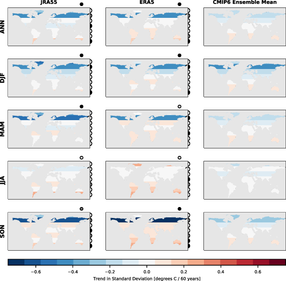
Figure 2. Maps of trends in daily temperature standard deviation by 20-degree latitude band, averaged annually and seasonally (rows) and for both reanalyses and the ALL ensemble mean (columns). The CMIP6 trend is calculated on the ensemble mean, giving equal weight to each model. For each reanalysis, circles are filled grey if the spatio-temporal ANT signal (from figure 3) is detected and black if it is consistent in magnitude with the reanalysis. Similarly, temporal results (from figure 4) are shown for each latitude band.
Download figure:
Standard image High-resolution imageTrends in daily temperature standard deviation for all of the forcing simulations used here are shown in figure S4. GHG forcing has very similar trend patterns to ALL forcing that are, in many cases, larger in magnitude. The AER forcing ensemble mean shows generally opposite trends to GHG, with increases in daily temperature standard deviation in the northern high latitudes, especially during the winter. The northern mid-latitudes show small decreases in standard deviation during SON from AER. Trends in the tropics and Southern Hemisphere are small for most forcings, though ALL and GHG show increases annually and during DJF and SON. Tends in the NAT ensemble mean are small in most latitude bands throughout the year.
As a comparison to the reanalysis, trends per latitude band for the GHCND observations are plotted in figure S5b. In addition, the ensemble mean model responses to each forcing are also included, processed and masked similarly to the observations. When compared to the reanalyses and the models processed without masking (figure S5a), large differences in the patterns are apparent. The models capture more reasonable values for the trend in the northernmost band (80–90∘ N) when using the full data, but not when masked by observational coverage. The full data show a consistent global pattern of near-zero trends from the NAT simulations and trends from AER that are smaller in magnitude, but opposite in sign from the trends due to GHG. This physically expected relationship is not realized when masking the data, which implies masked or missing data may hide the real pattern, providing additional justification for the use of reanalysis data in this paper instead of an observations dataset with incomplete coverage.
3.2. Detection and attribution
Scaling factors for a global spatio-temporal analysis of latitude-mean standard deviation are shown in figure 3 using the JRA55 reanalysis. Results for ERA5 are similar and shown in figure S6. The ANT signal is detected and consistent in magnitude with the reanalysis for standard deviation changes annually, as well as during all seasons except JJA (figure 3(a)). This ANT detection occurs even with the consideration of a NAT signal, but NAT is generally not detected.
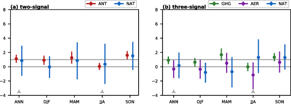
Figure 3. Scaling factors from a spatio-temporal detection and attribution of latitude-mean standard deviation for (a) two- and (b) three-signal analyses. Error bars represent the 90% uncertainty range. Upward (downward) grey arrows indicate model variability that is too large (small) according to a residual consistency test (see section 2.4), whereas the lack of an arrow indicates the test is passed.
Download figure:
Standard image High-resolution imageWith an anthropogenic signal detected, a three-signal analysis is used to attempt to separate GHG and AER forcing (figure 3(b)). The GHG signal is detected and consistent in magnitude with the reanalysis annually and for the same seasons where ANT was detected (DJF, MAM, SON). AER is not detected for any season. For most latitude bands, the trends in AER are of opposite sign to the trends in GHG (figure S4) and colinearity between the two may hinder the separation of the AER signal. As the NAT signal is weak, the uncertainty in the scaling factor is large. This is indicated by and explains the different NAT scaling factors between the two- and three-signal analyses.
The predominant feature of the spatio-temporal patterns is the strong decrease in the Northern Hemisphere during the cool season. This feature is found in both the reanalysis and the ALL and GHG model ensembles (figure S4) and explains the robust attribution for much of the year. In contrast, the trends during JJA are small and there is less agreement on the patterns between models and the reanalysis.
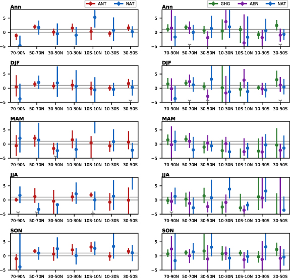
Scaling factors from the temporal analysis of latitude-mean standard deviation from each 20-degree band are shown in figure 4 for JRA55 and figure S7 for ERA5. The northern high latitudes (50–70∘ N) see detection of ANT with scaling factors consistent with one for annual, DJF, MAM, and SON. This result is consistent with Screen (2014) and Arctic amplification being an important driver of the changes. The higher latitudes (70–90∘ N) include much less land area and smaller signal-to-noise ratios may explain why a signal is not also detected for this band. In the tropics (10∘ S–10∘ N), the ANT signal is detected and consistent with one during JJA and SON. In the Southern Hemisphere mid-latitudes (30–50∘ S), the ANT signal is detected with scaling factors consistent with one annually and in DJF and SON. The GHG signal is detected and consistent in magnitude with the reanalysis for the northern high latitudes annually and in all seasons except JJA and for the southern mid-latitudes annually and in DJF.
Figure 4. Scaling factors from a temporal detection and attribution by latitude bands for two- (left) and three-signal (right) analyses by season (rows). See caption of figure 3 for additional details.
Download figure:
Standard image High-resolution image
For the temporal and spatio-temporal analyses, the results for all of the forcings are generally robust to the reanalysis (i.e. JRA55 or ERA5) and standard deviation calculation method used (i.e. if first removing the annual cycle). Most differences are in cases where an uncertainty range ends close to zero and small shifts can change the detection. The results for the transition seasons are consistent between the two calculation methods, except GHG is only detected in the spatio-temporal analysis for MAM when the full annual cycle is removed.
The ingest of satellite data by the reanalysis systems can lead to concerns regarding long-term homogeneity of the data. Although inhomogeneities are not apparent from the time series of latitude-band standard deviation, we also test the detection and attribution using only the satellite era (1980–2019). For the spatio-temporal analysis using this shorter period (figure S8), the ANT signal is detected and consistent with one annually and for DJF and MAM. The GHG signal is detected and consistent with one annually and for DJF and SON. For the temporal analysis using the shorter period (figure S9), the ANT signal is detected and consistent with one in the northern high latitudes (50–70∘ N) annually and for all seasons except JJA. The ANT signal is also detected annually and for DJF in the southern mid-latitudes (30–50∘ S) and for JJA in the tropics (10∘ S–10∘ N). We would expect less power to detect a signal with a shorter time period because there is less data and perhaps a weaker signal-to-noise ratio. However, there is still a credible signal using the shorter period and a majority of the detection results are consistent. Diagnosing an anthropogenic signal in both the shorter and longer periods increases our confidence in the results. In particular, we have more confidence for the annual and DJF attribution for the spatio-temporal analysis and the attribution annually and during DJF, MAM, and SON for the northern high latitudes (50–70∘ N). In addition, consistency also further demonstrates the suitability of the reanalyses.
4. Conclusions
The standard deviation of daily mean temperatures has decreased over the Northern Hemisphere high latitudes between 1960 and 2019 for annual and seasonal means over boreal winter, autumn, and spring. Weaker decreases are found for the Northern Hemisphere mid-latitudes for the annual mean and during winter. Small changes are found for the tropical region. In the Southern Hemisphere mid-latitudes, daily temperature standard deviation increased for the annual mean and during all seasons. The trends shown in this analysis are consistent with previous studies and physical understanding.
This manuscript presented new results for the detection and attribution of daily temperature variability. For global land areas, spatio-temporal changes in daily temperature variability are attributable to anthropogenic forcing. Attribution of an anthropogenic signal is found for annual values and in all seasons except boreal summer (JJA), likely influenced by the strong signal in the northern high latitudes. Additionally, the temporal changes in the northern high latitudes can be attributed to anthropogenic forcing on their own. Attributable increases in daily temperature standard deviation are also found for the Southern Hemisphere mid-latitudes.
Most of the attribution results presented here are generally robust to using different reanalyses, different time periods, and different methods of calculating variability. Consistent detection and attribution despite some changes in methodology speaks to the strength of the signal of anthropogenically-driven changes in daily temperature variability. Attributing observed changes in daily temperature variability to anthropogenic forcing provides further evidence that these changes will continue in the future with additional global warming. Species, ecosystems, and industries already sensitive to temperature variability may thus face additional challenges in the future.
Acknowledgments
We thank Francis Zwiers and Alex Cannon, as well as the editor and reviewers for their helpful comments. We also thank the providers of the observations, reanalysis products, and model simulations for making their data freely available.
Data availability statement
No new data were created or analysed in this study.