Arctic amplification of climate change: a review of underlying mechanisms

Michael Previdi; Karen L Smith; Lorenzo M Polvani

doi:10.1088/1748-9326/ac1c29

1. Introduction

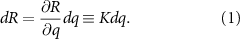
Arctic amplification (AA) of climate change is a prominent feature of the paleoclimatic record (Hoffert and Covey 1992, Miller et al 2010), present-day observations (Serreze et al 2009, Bekryaev et al 2010, Wang et al 2016, Richter-Menge et al 2019), and model projections of future climate (Intergovernmental Panel on Climate Change (IPCC) 2013, Davy and Outten 2020). AA refers to the enhancement of near-surface air temperature change in the Arctic relative to lower latitudes and the global mean, a feature that is readily apparent in observations over recent decades (figure 1(a)). Climate models from the fifth Coupled Model Intercomparison Project (CMIP5) reproduce the observed pattern of polar-amplified warming (figure 1(b)), although the models on average simulate less warming in the Arctic lower troposphere and more warming in the tropical lower troposphere (and thus weaker AA) compared to observations. CMIP5 models also simulate tropically-amplified warming in the upper troposphere that is not seen in observations (see also Po-Chedley and Fu 2012, Mitchell et al 2013, 2020, Santer et al 2013). We note, however, that the level of agreement between modeled and observed tropical tropospheric temperature trends may depend on the choice of observational dataset. For example, Santer et al (2017) found that observed trends based on one updated satellite dataset agreed well with the trends simulated by CMIP5 models.

Figure 1. Refer to the following caption and surrounding text. — **Figure 1.** (a) Latitude-pressure plot of 1979–2018 annual mean air temperature change (in K) based on linear trends (mean change of three atmospheric reanalyses: ERA5, JRA-55 and MERRA-2). (b) As in figure 1(a), but for the mean change of 12 CMIP5 models (bcc-csm1-1, CanESM2, CCSM4, CSIRO-Mk3-6-0, GFDL-CM3, inmcm4, IPSL-CM5A-LR, MIROC5, MPI-ESM-LR, MPI-ESM-MR, MRI-CGCM3 and NorESM1-M). For each model, 1979–2018 time series were created by concatenating the first ensemble member (r1i1p1) of the historical simulation with the first ensemble member of the RCP8.5 simulation. (c) Latitude-pressure plot of annual mean air temperature change (in K) based on the difference between the last 30 years of the CMIP5 abrupt 4 × CO₂ and pre- industrial control simulations (mean change of the 12 models listed in figure 1(b)). Note the different color scale in figure 1(c) compared to figures 1(a) and (b).
Download figure:
Standard image High-resolution image

Whatever the cause(s) of model-data differences (e.g. internal variability, model bias, observational uncertainty), these features of recent climate change are qualitatively consistent with the expected response to increases in atmospheric CO₂ (figure 1(c)). As will be discussed, however, AA is a robust response of the Earth system to climate forcing⁴ , and other forcings besides CO₂ very likely played a role in determining the magnitude of AA seen in recent decades (e.g. Najafi et al 2015, Polvani et al 2020). This polar-amplified warming has occurred in all seasons except boreal summer, with the strongest warming in fall and winter (figures 2(a) and (b)). Once again, this is in qualitative agreement with the expected response to CO₂ forcing (figure 2(c)).

Figure 2. Refer to the following caption and surrounding text. — **Figure 2.** (a) Observed 1979–2018 zonal mean surface air temperature (SAT) change (in K) for each season and the annual mean based on linear trends. Lines indicate the mean change of the three atmospheric reanalyses listed in figure 1(a), and shading denotes the ±1- sigma spread about this mean change (providing an estimate of observational uncertainty). (b) As in figure 2(a), but for the 12 CMIP5 models listed in the figure 1(b) caption (historical + RCP8.5 simulations). (c) As in figure 2(b), but for the SAT change based on the difference between the last 30 years of the abrupt 4 × CO₂ and pre-industrial control simulations. Note the different scale on the ordinate compared to figures 2(a) and (b).
Download figure:
Standard image High-resolution image

AA has had and will have important impacts on a range of human and natural systems, both within and outside the Arctic. Within the Arctic, enhanced warming and the associated melting of snow and ice present both challenges and opportunities to local human populations. Many communities face risks to food and water security as a result of changes in access to hunting areas and the distribution of traditional food sources, contamination of drinking water, changes in traditional food preservation methods, and increases in food contaminants (AMAP 2017, Osborne et al 2018). Additionally, the loss of snow and ice can create safety concerns as a result of damage and other alteration to infrastructure (e.g. roadways, buildings), and by leading to potentially dangerous conditions for hunting, recreation and other activities (e.g. Hovelsrud et al 2011, Schneider Von Deimling et al 2021). On the other hand, climate change offers some benefits to local communities such as increased opportunity for marine shipping, commercial fisheries, tourism, and access to resources as a result of the lengthening open water season in the Arctic Ocean (e.g. Melia et al 2016).

Natural systems within the Arctic are similarly affected by the pace and magnitude of climate warming. Changes in many animals' feeding, mating and migration habits are altering species distribution and abundance, introducing non-native species to the Arctic and in some cases threatening native species with extinction (CAFF 2013). Vegetation changes have also been observed in recent decades, including an overall 'greening' of the Arctic tundra that reflects an increase in plant growth and productivity (Osborne et al 2018). Arctic greening is an expected response to higher temperatures, although other factors such as moisture availability and the occurrence of extreme events (e.g. wildfires, insect outbreaks) will continue to play an important role in tundra vegetation dynamics (e.g. Wu et al 2020). Higher temperatures and the associated loss of sea ice are further driving increases in primary production by marine algae, as well as an expansion of harmful algal blooms that threaten human and ecosystem health (Osborne et al 2018).

The impacts of AA are by no means limited to the Arctic. Sea-ice loss, permafrost thaw, and other physical changes to the Arctic environment due to climate warming have the potential to significantly alter Arctic carbon cycling (e.g. McGuire et al 2009, Parmentier et al 2013, Schuur et al 2015, Natali et al 2019, Bowen et al 2020, Ito et al 2020, Bruhwiler et al 2021). This can impact the atmospheric concentrations of the well-mixed greenhouse gases CO₂ and methane, and thus the global climate forcing from these gases. Increases in global sea level due to melting of Arctic land ice are another important impact of Arctic warming (e.g. Shepherd et al 2012, Box et al 2018, Bamber et al 2019). This ice melt, along with projected increases in high-latitude precipitation and ocean warming, are expected to weaken the ocean's meridional overturning circulation (IPCC 2013), with implications for regional climate change and global ocean heat and carbon uptake. AA may also influence the atmospheric jet streams (both in the troposphere and stratosphere) in ways that lead to increased weather and climate extremes at midlatitudes (e.g. Francis and Vavrus 2012, Cohen et al 2014, Barnes and Screen 2015, Coumou et al 2018). However, the exact physical mechanisms involved, and the relative importance of Arctic warming compared to other influences (including internal variability), remain uncertain (e.g. McCusker et al 2016, Blackport and Screen 2020).

Despite this wide array of impacts, a clear consensus is still lacking within the scientific community as to which physical mechanisms are the most important in causing AA. Previous review articles addressing this topic were published by Miller et al (2010), Serreze and Barry (2011), and Walsh (2014). More recently, Goosse et al (2018) reviewed some of the key climate feedbacks in polar regions, and the methods for quantifying them. While AA was briefly discussed, it was not the focus of the article per se. Thus, the goal of the current article is to provide an up-to-date, focused review of the physical mechanisms that are likely responsible for AA: our review draws on the wealth of new research that has happened since the publication of earlier reviews. This will serve to synthesize our current understanding, and to identify remaining knowledge gaps and important paths for future research.

2. Methodology

Before beginning the formal review, we briefly describe our approach for identifying articles that were used as evidence in the review. Article selection began by searching for 'Arctic amplification' and then 'polar amplification' using both Web of Science and Scopus. For both databases, a document search for these phrases within the article title, abstract, and/or keywords was performed. Documents identified in this manner were then screened using the following four-step procedure:

(a)
Irrelevant documents unrelated to polar amplification as it pertains to climate change were eliminated. For example, an initial search for 'polar amplification' yielded multiple documents on topics as diverse as electronics and biology, which are clearly irrelevant to this review article.
(b)
Documents focused on polar amplification only in the Antarctic were eliminated. In addition to our review article being focused on the Arctic, there is evidence that the magnitude of polar amplification—as well as its governing physical processes—are different in the two hemispheres.
(c)
Opinion pieces and duplicate hits were eliminated.
(d)
Documents not focused on the physical processes driving AA were mostly eliminated. Two especially prevalent examples of such documents are: a) articles identifying the occurrence of AA (either in observations or climate model simulations) but not explicitly addressing its physical causes; and b) articles discussing the impacts of AA (e.g. on midlatitude weather and climate). While the main findings from some of these articles were touched upon above in the Introduction, the primary focus of our review is the causes of AA.

Articles that survived this elimination procedure were used as evidence in our review. These articles were supplemented with additional relevant articles that were identified by the authors while writing the review.

3. Physical mechanisms

We now commence with the formal review of the underlying physical mechanisms of AA. We begin with some notes on terminology (section 3.1), followed by discussion of the roles of climate forcing (section 3.2), climate feedbacks (section 3.3), and changes in poleward energy transport (PET) (section 3.4) in AA. The coupling between individual climate feedbacks, and between climate feedbacks and energy transport changes, is then discussed (section 3.5). Finally, a synthesis is provided at the end of the section (section 3.6). The important question of the dependence of forcing, feedbacks and energy transport on the state of the climate itself is considered in the next section (section 4).

3.1. Terminology

Throughout the discussion, we use the term climate forcing to refer to a change in an external driver of climate change, such as an increase in the atmospheric CO₂ concentration (see section 3.2 for other examples). The term radiative forcing is used to refer to the radiative flux change caused by a climate forcing. Radiative forcing without additional qualifiers refers to the radiative flux change at the top-of-atmosphere (TOA; Intergovernmental Panel on Climate Change (IPCC) 2013). However, we will also consider the surface radiative forcing and atmospheric radiative forcing, which denote, respectively, the radiative flux change at the surface, and the change in radiative flux divergence within the atmospheric column (i.e. the difference between the TOA and surface radiative forcing). In all cases, a positive (negative) forcing is one that induces warming (cooling).

In addition to the vertical level considered, radiative forcing can also be distinguished by whether or not the effects of rapid adjustments are included. A rapid adjustment is a response to a climate forcing that is driven directly by the forcing, independently of any change in the global mean surface temperature (Intergovernmental Panel on Climate Change (IPCC) 2013). When rapid adjustments are not included, the resulting radiative forcing is referred to as the instantaneous radiative forcing. In this case, the radiative flux change is due solely to the change in the climate forcing agent (e.g. the increase in atmospheric CO₂). Other types of radiative forcing include the radiative effects of one or more rapid adjustments. The stratosphere-adjusted radiative forcing includes the effect of stratospheric temperature adjustment, whereas the effective radiative forcing additionally includes the effects of other rapid adjustments (e.g. to tropospheric temperature, water vapor, and cloud cover). Additional discussion of these different types of radiative forcing can be found in Hansen et al (1997), Shine et al (2003), Hansen et al (2005), IPCC (2013), and Forster et al (2016), among others.

While rapid adjustments represent the temperature-independent part of the response to a climate forcing (see above), climate feedbacks are the part of the response that is dependent on global mean surface temperature change (Intergovernmental Panel on Climate Change (IPCC) 2013). In the discussion that follows, we will consider feedbacks associated with changes in surface and tropospheric temperatures⁵ (section 3.3.1), surface albedo (section 3.3.2), clouds and water vapor (section 3.3.3), and other properties of the Earth system (section 3.3.4). As for climate forcing, we will consider the impacts of climate feedbacks on the energy budget at both the TOA and surface. Positive (negative) feedbacks are those that reinforce (oppose) the effects of a climate forcing. Thus, for a positive forcing that induces warming, a positive feedback will lead to further warming.

Finally, we will consider changes in PET by the atmosphere (section 3.4.1) and ocean (section 3.4.2). While it is unclear whether PET changes can be classified as feedbacks (Goosse et al 2018), they are part of the response to climate forcing and are likely to contribute to AA, as will be discussed.

3.2. Climate forcing

The single most important climate forcing during the industrial era is increasing atmospheric CO₂ (Intergovernmental Panel on Climate Change (IPCC) 2013). AA as a response to increasing CO₂ was initially predicted by Arrhenius (1896), and, subsequently, much of the current understanding of AA has been gleaned from CO₂-forced climate model simulations (e.g. Manabe and Wetherald 1975, Manabe and Stouffer 1980, Holland and Bitz 2003, Winton 2006, Lu and Cai 2009a, Pithan and Mauritsen 2014, Previdi et al 2020). It seems appropriate then to begin our discussion of climate forcing with CO₂. AA is a robust response to CO₂ increases in the studies cited above (and many others). The first question we wish to address, therefore, is this: is AA caused by the direct radiative forcing from CO₂, or by subsequent responses within the climate system to this forcing?

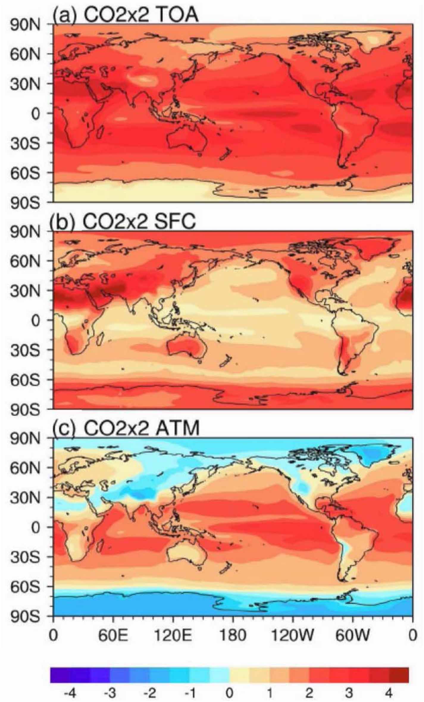
Figure 3 shows the instantaneous radiative forcing from doubling CO₂ at the TOA, the surface, and within the atmospheric column. At the TOA (figure 3(a)), CO₂ radiative forcing is largest at low latitudes and decreases toward the poles⁶ . This meridional structure is due to decreases in the climatological surface temperature and tropospheric vertical temperature gradient with latitude (Zhang and Huang 2014, Merlis 2015, Smith et al 2018), leading to the strongest enhancement of the greenhouse effect (and thus the largest radiative forcing) at low latitudes when CO₂ is increased.

Figure 3. Refer to the following caption and surrounding text. — **Figure 3.** Instantaneous radiative forcing (in W m⁻²) from doubling CO₂ as calculated by the rapid radiative transfer model (RRTM). The forcing is defined as the change in the net (i.e. longwave plus shortwave) downward radiative flux, and is shown for: (a) the top-of-atmosphere (TOA); (b) the surface (SFC); and (c) the atmospheric column (ATM, defined as TOA minus SFC). Adapted with permission from Huang *et al* (2017). © 2017. American Geophysical Union. All Rights Reserved.
Download figure:
Standard image High-resolution image

A qualitatively different picture emerges when one considers the CO₂ radiative forcing at the surface (figure 3(b)). In this case, the forcing is at a minimum at low latitudes and increases toward the poles. This is due to the overlap between CO₂ and water vapor absorption bands in the 12–18 μm spectral region. Because of this overlap, increases in the surface downwelling longwave radiation (DLR) are limited when CO₂ is increased, particularly at low latitudes where water vapor concentrations are highest and the emission from this spectral region is already largely saturated (Kiehl and Ramanathan 1982, Huang et al 2017).

The very different spatial patterns of CO₂ radiative forcing at the TOA and at the surface result in a strong latitudinal gradient in atmospheric radiative forcing (figure 3(c)), with positive forcing at low latitudes transitioning to negative forcing at the poles. This pattern of atmospheric radiative forcing has major implications for the PET, as will be discussed in section 3.4.1. To summarize, the impact of direct CO₂ radiative forcing on AA depends on perspective. From the perspective of the TOA and atmospheric column energy budgets (figures 3(a) and (c)), CO₂ radiative forcing opposes AA by preferentially heating the tropics. However, from the perspective of the surface energy budget (figure 3(b)), CO₂ radiative forcing contributes to AA by preferentially heating the Arctic.

While the discussion thus far has focused on CO₂, other climate forcings have also been shown to produce AA. These include changes in solar irradiance (Cai and Tung 2012, Stjern et al 2019), aerosols and aerosol precursors (Lambert et al 2013, Yang et al 2014, Najafi et al 2015, Acosta Navarro et al 2016, Chylek et al 2016, Sagoo and Storelvmo 2017, Conley et al 2018, Wang et al 2018, Stjern et al 2019, Kim et al 2019b), ozone-depleting substances (Polvani et al 2020), methane (Stjern et al 2019), and land use/land cover (van der Molen et al 2011, Lott et al 2020). The fact that AA occurs in response to these various forcings, with very different spatial, seasonal and spectral characteristics, suggests that it is a robust response to climate forcing that does not depend—at least existentially—on the details of the forcing. However, forcing details may impact the magnitude of AA. Modeling studies that have systematically varied the forcing latitude (Kang et al 2017, Park et al 2018, Stuecker et al 2018, Semmler et al 2020) and season (Bintanja and Krikken 2016) indicate that AA is likely to be strongest for high-latitude forcings, and for forcings occurring during spring and summer. What is clear though is that the direct effects of climate forcing alone are insufficient to fully understand AA (see also Virgin and Smith 2019). Such an understanding requires consideration of the feedback mechanisms operating within the climate system that act to amplify temperature changes at high northern latitudes. We discuss these feedbacks next.

3.3. Climate feedbacks

3.3.1. Temperature feedbacks

We begin our discussion of climate feedbacks with the temperature feedbacks that are associated with changes in surface and tropospheric temperatures. For ease of discussion, and for relevance to anthropogenic climate change, we consider a positive climate forcing that induces surface and tropospheric warming. The total temperature feedback at the TOA in response to such a forcing can be decomposed into contributions from vertically-uniform warming⁷ (Planck response) and changes in the tropospheric lapse rate (e.g. Hansen et al 1984, Bony et al 2006, Soden and Held 2006). The Planck response is the most fundamental mechanism acting to stabilize the climate, since surface and tropospheric warming will increase the outgoing longwave radiation (OLR) and thus oppose the effects of a positive forcing. However, because of the nonlinear dependence of OLR on temperature (as given by the Stefan–Boltzmann law), the Planck response is weaker (i.e. less stabilizing) over the colder Arctic relative to lower latitudes and to the global mean. In other words, OLR increases less over the Arctic than at lower latitudes, per degree of local warming, and this contributes to AA (Henry and Merlis 2019).

Globally averaged, changes in the tropospheric lapse rate are characterized by a reduction in the rate of temperature decrease with height, since the upper troposphere warms more than the lower troposphere and surface. Such a change in the temperature profile leads to a larger increase in OLR than would occur from the Planck response alone, representing a negative feedback on surface warming. However, the opposite occurs over the Arctic, where the upper troposphere warms less than the lower troposphere and surface. This opposes the basic Planck response and represents a positive feedback on surface warming. Thus, both the Planck and lapse rate components of the temperature feedback are expected to contribute to AA.

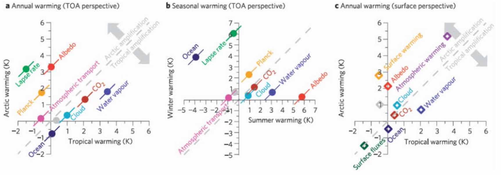
Indeed, previous studies that assessed contributions to Arctic warming and AA in both models (Langen et al 2012, Graversen et al 2014, Pithan and Mauritsen 2014, Payne et al 2015, Cronin and Jansen 2016, Previdi et al 2020, Zhang et al 2020) and observations (Hwang et al 2018, Zhang et al 2018) concluded that temperature feedbacks are important. Notably, Pithan and Mauritsen (2014) found that these feedbacks make the single largest contribution to AA in CMIP5 models subjected to an instantaneous quadrupling of atmospheric CO₂ (4 × CO₂). Their analysis demonstrates a prominent role for temperature feedbacks (and in particular the lapse rate feedback) both in causing AA in an annual mean sense (figure 4(a)), and also in producing the distinct seasonality in AA, with much stronger AA in winter relative to summer (figure 4(b); see also figure 2).

Figure 4. Refer to the following caption and surrounding text. — **Figure 4.** Warming contributions of individual feedback mechanisms calculated based on the difference between the last 30 years of the CMIP5 abrupt 4 × CO₂ and pre-industrial control simulations. (a) Arctic (60°–90° N) versus tropical (30° S–30° N) warming from a TOA perspective. (b) Arctic winter (December–January–February) versus summer (June–July–August) warming. (c) Arctic versus tropical warming from a surface perspective. For figures 4(a) and (c) feedbacks above the 1:1 line contribute to AA, whereas feedbacks below the line oppose AA. Grey is the residual error of the decomposition. 'Ocean' includes the effect of ocean transport changes and ocean heat uptake. Reprinted by permission from Springer Nature Customer Service Centre GmbH: Springer Nature, Nature Geoscience, Arctic amplification dominated by temperature feedbacks in contemporary climate models, Pithan and Mauritsen (2014).
Download figure:
Standard image High-resolution image

The effects of temperature feedbacks on the surface energy budget come from both surface warming and atmospheric warming, each of these contributing to AA (figure 4(c); see also Laîné et al 2016, Sejas and Cai 2016). The surface warming contribution arises because a larger increase in surface temperature is needed over the colder Arctic (relative to lower latitudes and to the global mean) to balance a given increase in downward energy flux (i.e. through enhanced surface emission of longwave radiation). This is fundamentally the same reason why latitudinal variations in the Planck response at the TOA contribute to AA. However, the effect is more pronounced when considering the surface energy budget, since the meridional temperature gradient at the surface is larger than that in the troposphere (Pithan and Mauritsen 2014). The atmospheric warming contribution to AA is associated with increases in the surface downwelling longwave radiation (DLR). These DLR increases are larger in the Arctic than at lower latitudes as a result of the much greater warming of the Arctic near-surface atmosphere (see figure 1).

3.3.2. Surface albedo feedbacks

As sea ice and snow cover retreat in a warming climate, the surface albedo (or reflectivity) decreases and a larger fraction of the incoming solar radiation is absorbed by the Earth system. Such surface albedo feedbacks therefore act to amplify surface warming, especially at high latitudes where sea ice and snow cover are most extensive. Changes in land ice (e.g. Hill et al 2014, Stap et al 2014, 2017, 2018) and vegetation (see also section 3.3.4) are additional sources of surface albedo change that may be important on long (multidecadal and longer) timescales. Here, however, we concentrate on the surface albedo (and related) feedbacks associated with the loss of sea ice and snow cover.

Those feedbacks have been shown to contribute to AA in both models (e.g. Budyko 1969, Sellers 1969, Manabe and Wetherald 1975, Manabe and Stouffer 1980, Hansen et al 1984, Holland and Bitz 2003, Hall 2004, Winton 2006, Crook et al 2011, Bintanja and van der Linden 2013, Baidin and Meleshko 2014, Graversen et al 2014, Pithan and Mauritsen 2014, Song et al 2014, Lang et al 2017, Sun et al 2018, Dai et al 2019, Duan et al 2019) and observations (e.g. Screen and Simmonds 2010a, 2010b, 2012, Pistone et al 2014, Hu et al 2017, Hwang et al 2018, Zhang et al 2018, 2019, Cai et al 2021, Yu et al 2021). For example, in their analysis of the CMIP5 4 × CO₂ simulations, Pithan and Mauritsen (2014) found that surface albedo feedbacks make the second largest contribution to AA, behind temperature feedbacks (figures 4(a) and (c)). The former were found to be important both in causing AA in a multimodel mean sense, and also in explaining the intermodel spread in the magnitude of AA (see also Boeke and Taylor 2018, Dai et al 2019, Block et al 2020, Hu et al 2020).

It is important to point out that surface albedo feedbacks are only active when sunlight is present, which is mainly in late spring and summer in the Arctic. AA itself, however, is absent in summer and is most pronounced in fall and winter (figure 2). How then can surface albedo feedbacks contribute to AA? To answer this question, it is necessary to consider the seasonal cycle of heat storage within the Arctic Ocean mixed layer (e.g. Chung et al 2021, Dai 2021). In a climatological sense, this seasonal cycle is characterized by ocean heat uptake in the late spring and summer, followed by a loss of heat from the ocean to the atmosphere in fall and winter. In a warming climate, the amplitude of this seasonal cycle is expected to increase, meaning greater ocean heat uptake in spring and summer and greater ocean heat loss in fall and winter (Carton et al 2015, figure 4(b)). This is a direct result of the loss of Arctic sea ice. In summertime, the surface albedo feedback associated with sea ice loss causes a greater amount of incoming solar radiation to be absorbed by the Arctic Ocean⁸ (Pistone et al 2014). Additionally, with less sea ice present, a larger fraction of the absorbed energy goes into increasing ocean temperatures rather than into melting ice (Carton et al 2015). The additional energy accumulated within the mixed layer in spring and summer is subsequently released to the atmosphere in fall and winter in the form of longwave radiation and latent and sensible heat. This process is facilitated by the loss of sea ice (area and thickness) in the latter seasons, and thus a weakening of the sea ice insulation effect.

The enhanced ocean-to-atmosphere energy exchange in fall and winter, which acts to warm the near-surface atmosphere, is now recognized to be of primary importance to AA (e.g. Screen and Simmonds 2010a, 2010b, Bintanja and van der Linden 2013, Sejas et al 2014, Yoshimori et al 2014a, Kim et al 2016, Franzke et al 2017, Boeke and Taylor 2018, Dai et al 2019, Chung et al 2021, Dai 2021). Its importance to observed AA in recent decades is suggested by the strong spatial correspondence between near-surface warming and sea ice loss over the Arctic, as shown in figure 5. This strong spatial correspondence further suggests a coupling between sea ice loss and the Arctic lapse rate feedback (e.g. Feldl et al 2020, Boeke et al 2021; see also section 3.5). The warming and moistening of the Arctic lower atmosphere increases the surface DLR, which hinders sea ice growth and thus helps to sustain the enhanced ocean-to-atmosphere energy flux (Burt et al 2016, Kim et al 2016, Alexeev et al 2017, Kim and Kim 2017, Kim et al 2019a).

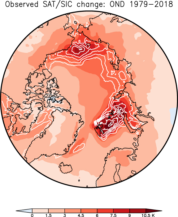
Figure 5. Refer to the following caption and surrounding text. — **Figure 5.** Observed Arctic SAT and sea ice concentration (SIC) changes during October–November–December (OND) 1979–2018 based on linear trends. SAT changes (in K; shading) are the mean of the three reanalyses listed in figure 1(a), and SIC changes (in %; white contours) are taken from the HadISST dataset version 1.1. For SIC changes, only negative values (corresponding to sea ice loss) are plotted using a contour interval of 10%; positive SIC changes during this period (greater than +10%) are limited to a small area between northeastern Greenland and Svalbard, and are omitted here for clarity.
Download figure:
Standard image High-resolution image

To summarize, there is considerable evidence that surface albedo feedbacks—and other feedbacks associated with the loss of sea ice and snow cover in a warming climate—make significant contributions to AA. It is worth noting, however, that polar-amplified warming has still been simulated in climate models even when surface albedo feedbacks (Hall 2004, Graversen and Wang 2009, Lu and Cai 2010, Graversen et al 2014) and all sea ice- and/or snow cover-related feedbacks (Schneider et al 1997, 1999, Alexeev 2003, Alexeev et al 2005, Duan et al 2019) have been eliminated (e.g. by fixing the surface albedo). This suggests that other processes are capable of producing AA, even in the absence of any changes in surface albedo and/or sea ice/snow cover. The importance of temperature feedbacks for AA was discussed above in section 3.3.1. However, other processes may also be important. For example, Graversen and Wang (2009) linked AA in their model to a stronger greenhouse effect over the Arctic resulting from increases in clouds and water vapor, and Alexeev et al (2005) emphasized the importance of increased atmospheric PET. We discuss cloud and water vapor feedbacks in more detail in the next section, and atmospheric PET changes will be considered in section 3.4.1.

3.3.3. Cloud and water vapor feedbacks

Most climate models project that the Arctic will become cloudier in a warmer climate (Vavrus 2004, Vavrus et al 2009, 2011, Taylor et al 2013), mainly due to increases in low clouds in fall and winter. This result is supported by analyses of observed cloud changes in recent decades (Wu and Lee 2012, Jun et al 2016, Cao et al 2017, Philipp et al 2020). Some modeling studies also indicate that Arctic middle and high clouds may increase as well (Vavrus et al 2009, 2011). Increases in Arctic low clouds in fall and winter are a direct response to sea ice loss, which acts to destabilize the boundary layer and enhance moisture availability and boundary-layer convection (Kay and Gettelman 2009, Vavrus et al 2009, Eastman and Warren 2010, Palm et al 2010, Vavrus et al 2011, Wu and Lee 2012, Abe et al 2016, Jun et al 2016, Morrison et al 2019, Philipp et al 2020). In contrast, sea ice loss seems to have an insignificant impact on Arctic cloud cover during summer (Kay and Gettelman 2009, Morrison et al 2019, Choi et al 2020).

Given that low cloud increases occur mainly during fall and winter when insolation is at a minimum over the polar cap, the associated radiative effects occur primarily in the longwave portion of the spectrum. However, these effects differ considerably at the TOA and surface (Pithan and Mauritsen 2014). At the TOA, low cloud increases have a relatively small impact on OLR since the temperature of these clouds is not that different from the surface temperature. In contrast, these cloud increases strongly enhance the emissivity of the Arctic lower troposphere and thus the surface DLR (Vavrus et al 2011, Taylor et al 2013, Abe et al 2016, Jun et al 2016, Cao et al 2017, Morrison et al 2019, Philipp et al 2020). These DLR increases, which may be further enhanced by cloud phase changes (i.e. a larger liquid-to-ice ratio; Tan and Storelvmo 2019, Huang et al 2021), contribute to additional surface warming and sea ice melt (Vavrus et al 2011, Cao et al 2017, Philipp et al 2020), and may also help to suppress the formation of Arctic air masses over high-latitude continents (Cronin and Tziperman 2015, Cronin et al 2017).

Understanding the effect of cloud feedbacks on AA requires consideration of the meridional structure of these feedbacks. In other words, it is important to also consider cloud feedbacks outside of the Arctic. Globally averaged, the net (i.e. longwave plus shortwave) cloud feedback is positive in most current climate models, but with large intermodel spread mainly due to differences in shortwave cloud feedback (Zelinka et al 2020). This suggests that the effect of cloud feedbacks on AA is likely to be model dependent. Additionally, this effect depends on whether one considers changes to the TOA energy budget, or to the surface energy budget. From a TOA perspective, cloud feedbacks oppose AA in the CMIP5 multimodel mean (figure 4(a)), whereas they contribute to AA from a surface perspective (figure 4(c)). (Note that in both cases, however, the magnitude of the cloud contribution is relatively small; see also Middlemas et al (2020).) This difference in the inferred cloud effect is partly due to the greater impact of Arctic cloud changes on the longwave radiation at the surface, as discussed above. Cloud feedbacks (and thus the cloud contribution to AA) estimated from observations in recent decades are similarly uncertain, these estimates depending on the choice of observational datasets, the time period considered, and the method used to quantify cloud feedbacks (Zhang et al 2018).

Now we turn to water vapor feedbacks: these are positive in the Arctic at both the TOA and surface, with water vapor increases in the Arctic lower troposphere being an important contributor to increases in surface DLR (Chen et al 2011, Ghatak and Miller 2013, Cao et al 2017). However, water vapor feedbacks in the tropics (and in the global mean) tend to be stronger than they are in the Arctic, both at the TOA and surface, and thus the direct effect of these feedbacks is to oppose AA (figures 4(a) and (c)). In order to understand why water vapor feedbacks in the tropics tend to be stronger, we decompose the difference in the tropical (30° S–30° N) and Arctic (60°–90° N) mean water vapor feedbacks in the CMIP5 abrupt 4 × CO₂ simulations. We express the water vapor feedback dR as the product of two terms (see Soden et al 2008): a radiative kernel K, describing the sensitivity of the TOA or surface radiation to incremental changes in specific humidity, and a climate response dq, defined here as the difference in specific humidity between the last 30 years of the CMIP5 abrupt 4 × CO₂ and pre-industrial control simulations, i.e.

$\begin{align}dR = \frac{{\partial R}}{{\partial q}}dq \equiv Kdq.\end{align} \tag{ 1 }$

The difference in water vapor feedback ΔdR between the tropics and Arctic can then be written as:

$\begin{align}\Delta dR = dq\Delta K + K\Delta dq + \Delta K\Delta dq\end{align} \tag{ 2 }$

where dqΔK and KΔdq represent the contributions to ΔdR from meridional differences in K and dq, respectively, and ΔKΔdq is the nonlinear term representing the covariance between K and dq.

Figure 6 shows the various terms in equation (2) for both the TOA (figure 6(a)) and surface (figure 6(b)) water vapor feedbacks. We find that ΔdR is 1.71 ± 0.63 K (multimodel mean ± 1σ) at the TOA, and 0.67 ± 0.24 K at the surface. This TOA value is similar to the one found by Pithan and Mauritsen (2014) (compare figures 4(a) and 6(a)), although our kernel (Previdi 2010, Previdi and Liepert 2012) yields a somewhat smaller value of ΔdR at the surface (compare figures 4(c) and 6(b)).

Figure 6. Refer to the following caption and surrounding text. — **Figure 6.** Decomposition of the difference in tropical (30° S–30° N) and Arctic (60°–90° N) mean water vapor feedback at the (a) TOA and (b) surface in the CMIP5 abrupt 4 × CO₂ simulations (blue bars represent the multimodel mean of the 12 CMIP5 models listed in the figure 1(b) caption, with black error bars bracketing ± 1σ about the mean). Labels along the abscissa are the terms in equation (2) (see discussion in text). Water vapor feedbacks are calculated using radiative kernels from ECHAM5 (Previdi 2010, Previdi and Liepert 2012), and are expressed as warming contributions (or partial temperature changes) as in figure 4.
Download figure:
Standard image High-resolution image

The decomposition of ΔdR (equation (2)) produces qualitatively similar results at the TOA and surface (figure 6). We find that in both cases, the stronger water vapor feedback in the tropics compared to the Arctic can be explained by the larger increase in specific humidity in the former (i.e. by the KΔdq term). This larger increase in specific humidity is due to the strong (and nonlinear) dependence of the saturation vapor pressure on temperature—as given by the Clausius–Clapeyron relationship—which leads to the largest increases in water vapor amounts where the climatological temperatures are highest (i.e. in the tropics). Note though that KΔdq is largely offset by dqΔK and ΔKΔdq (particularly the latter). This offset reflects an overall lower radiative sensitivity to water vapor perturbations (as measured by K) in the tropics compared to the Arctic, owing to the greater saturation of water vapor emission under moist tropical conditions. The lower radiative sensitivity in the tropics leads to significantly smaller values of TOA and surface ΔdR than would result from meridional differences in dq alone.

To summarize, stronger tropical than Arctic water vapor feedbacks in the CMIP5 abrupt 4 × CO₂ simulations can be explained by larger increases in specific humidity in the tropics. The greater tropical moistening outweighs the opposing effect of lower tropical radiative sensitivity to water vapor changes. In addition to these implications for water vapor feedback, larger specific humidity increases in the tropics compared to the Arctic also lead to enhanced poleward moisture transport with climate warming. As will be discussed below (see section 3.4.1), this enhanced moisture transport is now recognized to be important for AA.

3.3.4. Other feedbacks

To conclude this section, we briefly discuss a few other feedbacks that have been suggested to contribute to AA. One of these involves the northward shift of boreal forest and overall greening of the Arctic that are expected to occur with climate warming (see section 1). These vegetation changes enhance Arctic surface warming directly by reducing the surface albedo of high latitude land areas, and thus increasing the surface absorption of solar radiation. Further enhancement of Arctic warming may also occur indirectly through interactions between vegetation changes and changes in water vapor, clouds and sea ice (O'ishi and Abe-Ouchi 2011, Jeong et al 2014, Willeit et al 2014, Chae et al 2015, Cho et al 2018, Park et al 2020). Increases in phytoplankton biomass in the Arctic may produce an additional positive feedback on surface warming, by enhancing solar radiation absorption within the ocean surface layer (Park et al 2015).

These changes in the biosphere affect not only the surface solar radiation, but also other surface fluxes such as the turbulent fluxes of latent and sensible heat (e.g. evapotranspiration changes due to vegetation change). More generally, it is important to consider the possible impact of changes in the surface turbulent energy fluxes on AA, in addition to the surface radiative flux changes discussed in some detail above. In a warming climate, the turbulent energy (latent plus sensible heat) transfer from the surface to the atmosphere is generally expected to increase (e.g. Cai and Lu 2007, Taylor et al 2013). Increases in the surface latent heat flux (or evaporation) tend to be largest at low latitudes (particularly over oceans), a consequence of the strong temperature dependence of the saturation vapor pressure (i.e. the Clausius–Clapeyron relationship). These evaporation increases at low latitudes provide a strong negative feedback on surface warming, acting to stabilize tropical sea surface temperatures, and thus contributing to AA (Newell 1979, Hartmann and Michelsen 1993, Cai and Lu 2007, Yoshimori et al 2014b).

3.4. Changes in PET

3.4.1. Atmospheric transport

In section 3.2, we discussed the difference in the latitudinal structure of CO₂ radiative forcing at the TOA and surface. Recall that, at the TOA, the forcing is at a maximum in the tropics and decreases toward the poles (figure 3(a)). At the surface, however, this latitudinal gradient is reversed, with the maximum forcing occurring at high latitudes (figure 3(b)). This difference between the TOA and surface leads to an even stronger latitudinal gradient in CO₂ radiative forcing within the atmosphere, with the forcing acting to heat the atmosphere in the tropics and generally cool it in polar regions (figure 3(c)). Such a forcing pattern contributes to an increase in the atmospheric PET (e.g. Cai 2006, Huang et al 2017), which redistributes the additional energy that is gained at low latitudes. In accordance with this, coupled climate models forced with increased CO₂ robustly simulate increases in atmospheric PET in the midlatitudes of both hemispheres (Held and Soden 2006, Hwang and Frierson 2010, Wu et al 2011, Zelinka and Hartmann 2012, Huang and Zhang 2014, Armour et al 2019).

Over the Arctic, however, model responses are not so robust. While some models simulate increases in atmospheric PET into the Arctic, other models simulate decreases (figure 7(a); see also figure 3 in Pithan and Mauritsen 2014). Decreases in atmospheric PET into the Arctic have also been reported in observations over recent decades (Sorokina and Esau 2011, Fan et al 2015), although the magnitude and sign of the PET change are sensitive to the dataset (Liu et al 2020), time period (Graversen 2006, Yang et al 2010), and Arctic sector (Mewes and Jacobi 2019) considered. From an energetic perspective, such PET decreases imply that the net effect of local feedbacks over the Arctic must be to heat the atmospheric column, thus balancing the cooling effects from reduced PET and CO₂ radiative forcing. This further implies a coupling between local feedbacks and PET changes, which will be discussed in section 3.5.

Figure 7. Refer to the following caption and surrounding text. — **Figure 7.** Changes in northward energy transports (in PW) in CMIP3 models (see legend) from 2001–2020 to 2081–2100 in the A2 scenario: (a) atmospheric energy transport; (b) moisture (solid) and dry static energy (DSE; dashed) transport; and (c) oceanic energy transport. Reproduced with permission from Hwang *et al* (2011). Copyright 2011 by the American Geophysical Union.
Download figure:
Standard image High-resolution image

The total change in atmospheric PET can be decomposed into a change in dry static energy (DSE) transport, and a change in moisture transport. While the total change in PET into the Arctic is not robust across model simulations—as noted above—the changes in the DSE and moisture transports individually are robust. DSE transport into the Arctic decreases with climate warming, while moisture transport into the Arctic increases (figure 7(b)). The sign of the total PET change is primarily determined by the magnitude of the decrease in DSE transport. In models with strong decreases in DSE transport, the total PET into the Arctic also decreases. However, in models with weak decreases in DSE transport, the increase in moisture transport (which has comparatively little intermodel spread; see figure 7(b)) results in an increase in the total PET.

Decreases in DSE transport into the Arctic are a response to reductions in the meridional temperature gradient due to polar-amplified warming (e.g. Langen and Alexeev 2007, Hwang et al 2011, Skific and Francis 2013, Graversen and Burtu 2016, Audette et al 2021). The relationship between the DSE transport and the meridional temperature gradient leads to a negative correlation between AA and the transport change in climate models: models with the largest AA also tend to have the largest decrease in DSE (and total) transport (Hwang et al 2011). We emphasize that this correlation reflects the response of the atmospheric PET to AA. However, PET changes are also likely to be an important cause of AA, as will be discussed.

Increases in moisture transport into the Arctic are a response to a stronger meridional gradient of specific humidity (e.g. Graversen and Burtu 2016; see also section 3.3.3). Several studies have emphasized the importance of this enhanced moisture transport for AA (e.g. Flannery 1984, Cai 2005, Cai and Lu 2007, Langen and Alexeev 2007, Graversen and Burtu 2016, Yoshimori et al 2017, Merlis and Henry 2018, Graversen and Langen 2019). Graversen and Burtu (2016) demonstrated using reanalysis data that a given increase in moisture transport across 70° N results in a greater Arctic surface warming than an equivalent increase in the DSE transport. This occurs because the increase in moisture transport acts to strengthen the greenhouse effect over the Arctic—both directly and by enhancing Arctic cloudiness—leading to large increases in the surface DLR (see also Rodgers et al 2003, Gong et al 2017, Kim and Kim 2017, Praetorius et al 2018, Hao et al 2019, Clark et al 2021, Dunn-Sigouin et al 2021). Thus, the warming effect from enhanced moisture transport into the Arctic with climate change can outweigh the cooling effect from reduced DSE transport, leading to a net Arctic warming from atmospheric PET changes even when the total PET decreases (Graversen and Burtu 2016, Graversen and Langen 2019).

Changes in PET are the means by which heating anomalies outside the Arctic can influence the Arctic climate. Previous studies have emphasized the importance of heating anomalies in Northern Hemisphere (NH) midlatitudes (Solomon 2006, Laliberté and Kushner 2013, Fajber et al 2018), and in the tropics (Rodgers et al 2003, Lee et al 2011, Yoo et al 2011, Lee 2014, Baggett and Lee 2015, Baggett et al 2016, Baggett and Lee 2017, Yim et al 2017, Baxter et al 2019, McCrystall et al 2020, Dunn-Sigouin et al 2021). For instance, it has been suggested (Laliberté and Kushner 2013, Fajber et al 2018) that near-surface temperature and moisture anomalies at midlatitudes are propagated by synoptic-scale eddies along moist isentropes to the Arctic midtroposphere. This would imply a direct influence of midlatitude surface warming on the lapse rate and water vapor feedbacks over the Arctic, with implications for Arctic surface warming and AA. Alternatively, changes in atmospheric PET into the Arctic may be induced by heating anomalies in the tropics. For instance, it has been suggested that enhanced localized convection over the Maritime Continent can trigger poleward-propagating Rossby waves that may enhance PET into the Arctic and contribute to AA (Lee et al 2011, Yoo et al 2011, Lee 2014, Baggett and Lee 2015, Baggett et al 2016, Baggett and Lee 2017). PET into the Arctic could also be enhanced by a northward shift of the Inter-tropical Convergence Zone, which many models project will occur with climate warming (Yim et al 2017).

The relative importance of heating anomalies in the tropics versus the midlatitudes has implications for how we view changes in atmospheric PET. If tropical heating anomalies are more important, a better understanding of changes in tropical convection would be critical for understanding atmospheric PET changes. On the other hand, if midlatitude heating anomalies are more important, one might wish to place greater emphasis on better understanding the dynamics of the eddy-driven jets and storm tracks. In addition to these considerations, it is also worth noting that tropical and midlatitude heating anomalies have different preferred teleconnection pathways to the Arctic, meaning that their relative importance is likely to be regionally dependent (Ye and Jung 2019, Hall et al 2021).

3.4.2. Oceanic transport

We now consider changes in PET by the ocean. In response to climate warming, models generally simulate decreases in oceanic PET at NH midlatitudes, and increases in oceanic PET into the Arctic (figure 7(c); Holland and Bitz 2003, Bitz et al 2006, Held and Soden 2006, Hwang et al 2011, Kay et al 2012, Graham and Vellinga 2013, Koenigk et al 2013, Koenigk and Brodeau 2014, Koenigk and Brodeau 2017, Nummelin et al 2017, Singh et al 2017, 2018, Docquier et al 2019, van der Linden et al 2019, Beer et al 2020). Increased oceanic PET into the Arctic in recent decades has also been inferred from ocean temperature reconstructions based on marine sediments off Western Svalbard (Spielhagen et al 2011). Modeling studies (Singh et al 2017, 2018) examining the seasonality of oceanic PET changes have found that enhanced oceanic PET into the Arctic in the annual mean is the result of PET increases during boreal winter, with summertime PET into the Arctic decreasing slightly. In addition to oceanic PET increases, enhanced vertical ocean heat flux into the Arctic Ocean mixed layer is also simulated by models in response to climate warming (Graham and Vellinga 2013).

These changes in the oceanic energy transport are understood to varying degrees. The simulated decrease in oceanic PET at NH midlatitudes is mainly the result of a weakening of the Atlantic meridional overturning circulation with climate warming (e.g. Gregory et al 2005, Cunningham and Marsh 2010, Hwang et al 2011, Nummelin et al 2017). At higher latitudes, however, the cause(s) of the increase in oceanic PET into the Arctic is less certain. In particular, it is unclear to what extent this increase is driven by circulation changes, versus the advection of ocean heat anomalies by the background flow. Bitz et al (2006) examined simulations from a coupled atmosphere-ocean model forced with increasing CO₂, and found that oceanic PET into the Arctic was enhanced largely as a result of strengthened inflow driven by increased convection along the Siberian shelves. This increased convection, in turn, was driven by enhanced sea ice production and ocean-to-atmosphere heat flux in winter. However, other studies with coupled models have found that the role of circulation changes is small, and that oceanic PET increases are largely due to the advection of warmer water into the Arctic by the background flow (Koenigk and Brodeau 2014, Nummelin et al 2017). Nummelin et al (2017) linked this to reduced heat loss from the subpolar ocean to the atmosphere, which increases the heat content of the water masses that are advected into the Arctic.

In addition to possible model dependence, the relative importance of circulation changes versus passive temperature advection for oceanic PET changes is likely to vary with time, as patterns of ocean heat uptake and other aspects of the climate response evolve. For example, strengthened oceanic inflow to the Arctic driven by increased convection along the Siberian shelves is expected to eventually diminish in a much warmer climate as wintertime sea ice production declines (Bitz et al 2006). Sea ice declines are also key to understanding the enhanced vertical ocean heat flux into the Arctic Ocean mixed layer noted above. Specifically, as sea ice melts, the wind stress on the Arctic Ocean surface increases. This enhances upper ocean mixing and entrains warmer water from depth into the mixed layer (Graham and Vellinga 2013).

While some of the additional energy delivered to the mixed layer through ocean transport changes goes into warming the mixed layer, most of this additional energy goes into melting sea ice and warming the near-surface atmosphere (Bitz et al 2006, Koenigk and Brodeau 2014, Marshall et al 2015, Docquier et al 2019, Alkama et al 2020a). This suggests a positive contribution from ocean transport changes to AA (Holland and Bitz 2003, Hwang et al 2011, Mahlstein and Knutti 2011, Graham and Vellinga 2013, Koenigk and Brodeau 2014, Marshall et al 2014, 2015, Nummelin et al 2017, Singh et al 2017, 2018, Beer et al 2020). It is worth emphasizing that this positive contribution occurs during winter (figure 4(b)), the time of year when oceanic PET into the Arctic is enhanced (Singh et al 2017, 2018), and when the ocean is a net source of heat for the atmosphere (section 3.3.2). The contribution of ocean transport changes to Arctic warming and sea ice melt exemplifies the coupling between PET changes and local feedbacks, a topic that will be discussed further in the next section.

3.5. Coupling between mechanisms

Thus far, we have considered the contributions of climate forcing (section 3.2), climate feedbacks (section 3.3), and PET changes (section 3.4) to AA. While these contributions have been discussed separately, it is now recognized that the physical mechanisms involved are closely coupled with one another. In this section, we discuss the possible couplings between mechanisms, and their implications for our understanding of AA.

Some examples of coupling have already been mentioned. For instance, in sections 3.3.2 and 3.3.3, we noted that Arctic sea ice loss leads to enhanced ocean-to-atmosphere heat flux in the fall and winter. This is associated with a warming and moistening of the boundary layer, and increases in low-level clouds, which implies an impact of sea ice loss on the lapse rate, water vapor, and cloud feedbacks over the Arctic. The water vapor and cloud feedbacks are further impacted by increases in poleward moisture transport (section 3.4.1), and sea ice loss is enhanced by increases in oceanic PET into the Arctic (section 3.4.2). Changes in atmospheric PET are also known to play an important role in modulating the Arctic lapse rate feedback (Graversen et al 2008, Screen et al 2012, Laliberté and Kushner 2013, Cronin and Jansen 2016, Feldl et al 2017a, Fajber et al 2018, Kim et al 2018, Park et al 2018, Kim and Kim 2019, Feldl et al 2020).

The interactions between these physical mechanisms work in both directions. For example, increases in Arctic lower tropospheric temperature, moisture and cloud cover resulting from sea ice loss act to strongly enhance the surface DLR, thus contributing to even greater ice loss (sections 3.3.2 and 3.3.3). Additionally, local feedbacks over the Arctic that are partly determined by PET changes modify the energy balance and thus affect the PET (Hwang et al 2011, Feldl and Roe 2013, Merlis 2014, Huang et al 2017, Yoshimori et al 2017, Feldl et al 2017b). The effect of a particular feedback on PET depends on the meridional gradient of heating induced by that feedback. Feedbacks that preferentially heat the Arctic relative to lower latitudes—such as the surface albedo feedback—act to decrease the PET into the Arctic. In contrast, feedbacks that preferentially heat lower latitudes—such as the water vapor feedback (see section 3.3.3)—act to increase the PET. This is the same line of reasoning used to explain the increase in atmospheric PET induced by CO₂ radiative forcing (see section 3.4.1). In some coupled models, this direct CO₂ effect is overwhelmed by an opposite-signed effect from climate feedbacks, resulting in a decrease in atmospheric PET into the Arctic (figure 7(a)).

The coupling between physical mechanisms that is described here has important implications. For instance, modeling studies suggest that nonlinear interactions between local feedbacks will act to warm the Arctic more than lower latitudes, thus contributing to AA (Feldl and Roe 2013, Södergren et al 2018). Such nonlinear interactions—though not fundamental to the occurrence of AA—have been ignored in traditional linear climate feedback analysis⁹ . Additionally, the perceived contribution of a particular physical mechanism to AA can change—at times qualitatively—when its effects on other mechanisms are taken into account. For example, when considering only direct effects on the TOA radiation, both CO₂ forcing and water vapor feedback oppose AA, since they preferentially heat the tropics (figure 4(a)). However, when their effects on the atmospheric PET are taken into account (see above), they both contribute to AA (Russotto and Biasutti 2020). Such coupling between physical mechanisms—and whether or not it is accounted for—can partly explain why previous studies have sometimes reached different (and even contradictory) conclusions about the main causes of AA.

3.6. Synthesis of physical mechanisms

To conclude section 3, we present a brief synthesis of the studies that we have reviewed in table 1. For each of the physical mechanisms discussed above, we tabulate the total number of studies N that assessed the contribution of that mechanism to AA. We then calculate the percentages of N that are positive (mechanism contributes to AA), negative (mechanism opposes AA), and positive or negative (mechanism either contributes to or opposes AA¹⁰ ). The physical mechanisms considered in this synthesis include the following: CO₂ forcing, temperature feedbacks (including Planck response and lapse rate feedback), surface albedo feedbacks (including sea ice albedo/insulation effects and other (snow cover, land ice, and vegetation) surface albedo feedbacks), cloud feedbacks, water vapor feedbacks, surface evaporation feedbacks, biosphere feedbacks, atmospheric PET changes, and oceanic PET changes.

Table 1. Synthesis of physical mechanisms. For each of the mechanisms listed, N indicates the total number of studies that assessed the contribution of that mechanism to AA. The percentages of N that are positive (mechanism contributes to AA), negative (mechanism opposes AA), and positive or negative (mechanism either contributes to or opposes AA) are also given.

Physical mechanism	N	% +	% −	% ±
CO₂ forcing	29	34	48	18
Temperature feedbacks Planck response Lapse rate feedback	34 23 29	100 100 100
Surface albedo feedbacks Sea ice albedo/insulation effects Other surface albedo feedbacks	81 66 35	100 100 100
Cloud feedbacks	40	55	25	20
Water vapor feedbacks	37	32	62	6
Surface evaporation feedbacks	10	90		10
Biosphere feedbacks	8	88		12
Atmospheric PET changes	78	78	8	14
Oceanic PET changes	28	75	11	14

Table 1 suggests that these physical mechanisms can be grouped into three categories. The first category includes mechanisms with relatively large N and a high level of agreement between studies on the sign of the mechanisms' contribution to AA. In this category, we include temperature feedbacks (section 3.3.1), surface albedo feedbacks (section 3.3.2), atmospheric PET changes (section 3.4.1), and oceanic PET changes (section 3.4.2). The studies we reviewed largely agree (for atmospheric/oceanic PET changes) or unanimously agree (for temperature/surface albedo feedbacks) that these mechanisms contribute positively to AA (often making a leading-order contribution).

The second category includes mechanisms with relatively large N, but with a lower level of agreement between studies on the sign of the mechanisms' contribution to AA. This category includes CO₂ forcing (section 3.2), and cloud and water vapor feedbacks (section 3.3.3). Nearly half (48%) of the studies surveyed found that direct CO₂ forcing opposes AA. The majority (62%) of the studies surveyed found that water vapor feedback also opposes AA, while a slightly smaller majority (55%) found that cloud feedback contributes to AA. For each of these mechanisms, however, smaller but significant percentages of the studies surveyed inferred an opposite-signed contribution (e.g. about a third of the studies found a positive contribution to AA from direct CO₂ forcing and water vapor feedback).

The third and final category includes mechanisms with small N and a high level of agreement between studies. This category includes surface evaporation and biosphere feedbacks (section 3.3.4). There is strong (∼90%) agreement that these mechanisms contribute positively to AA, but this is based on a relatively small number of studies (N⩽ 10).

Based on these results, we can conclude that the physical mechanisms included in the first category (temperature/surface albedo feedbacks and atmospheric/oceanic PET changes) likely contribute positively to AA. For the mechanisms included in the second category (CO₂ forcing and cloud/water vapor feedbacks), the sign of the contribution to AA is more uncertain given the lower level of agreement between studies. Different studies may infer opposite-signed contributions from these mechanisms depending, for example, on the choice of climate model, whether the TOA or surface energy budget is considered, and whether effects on the energy transport are accounted for (see discussion above). Finally, the physical mechanisms included in the third category (surface evaporation and biosphere feedbacks) may contribute positively to AA, but given their small value of N (see table 1), it is important that this positive contribution be confirmed through additional studies. This is particularly true for biosphere feedbacks, which have been studied far less than physical feedbacks (at least in terms of their potential contribution to AA).

4. Climate state dependence

From the preceding discussion, it should already be clear that several changes occurring within the Earth system in response to climate forcing—including both local feedbacks and PET changes—are important in producing AA. We argue here that some of the most important changes are a direct consequence of the climate state at the time the forcing is imposed.

The first aspect of the climate state that we will consider is the meridional temperature gradient. The existence of a strong meridional temperature gradient in the present climate is the reason why the Planck response contributes to polar-amplified warming (section 3.3.1). In other words, colder polar regions must warm more than lower latitude regions in order to balance a given magnitude (positive) radiative forcing through enhanced OLR. Additionally, the meridional temperature gradient partly explains why a given increase in atmospheric CO₂ concentration produces the largest radiative forcing at low latitudes (section 3.2). The associated meridional gradient in heating drives an increase in atmospheric PET (section 3.4.1), which contributes to AA. Even with spatially-uniform heating, however, an increase in atmospheric PET is still expected as a result of enhanced moisture transport (e.g. Langen and Alexeev 2007, Merlis and Henry 2018). The increase in moisture transport is a response to a stronger meridional gradient in specific humidity (section 3.4.1). This is another consequence of the meridional temperature gradient—as well as the nonlinear dependence of the saturation vapor pressure on temperature (i.e. the Clausius-Clapeyron relationship)—which conspire to produce the largest increases in specific humidity at low latitudes as the climate warms (section 3.3.3).

In addition to the meridional temperature gradient, the climatological vertical temperature structure of the atmosphere is also important for AA. The climatological near-surface inversion over the Arctic strongly suppresses vertical mixing and thus confines surface heating anomalies to the lowermost atmosphere, leading to a positive lapse rate feedback (figures 4(a) and (b); see also Lauer et al 2020, Previdi et al 2020). In contrast, the more unstable tropical atmosphere permits deep vertical mixing by convection which efficiently transports heat to the upper troposphere, leading to a negative lapse rate feedback (figure 4(a)). At these upper tropospheric levels where the atmosphere above is optically thin, the heat is readily lost to space as OLR. This again is in stark contrast to what occurs in the Arctic, where heating anomalies trapped near the surface hardly contribute to the TOA OLR (Bintanja et al 2011). Instead, these heating anomalies primarily enhance the surface DLR, thus amplifying the Arctic surface warming. In summary, differences in the climatological static stability between the polar and tropical atmospheres lead to marked differences in the efficiency of vertical mixing, and, therefore, in the efficiency of longwave energy loss to space. In this regard, AA can be viewed as a manifestation of the relative inefficiency of the Arctic climate system in ridding itself of excess heat.

Lastly, we consider the importance of the climatological Arctic sea ice. Holland and Bitz (2003) examined simulations from several CMIP2 climate models, and found that climatological sea ice conditions in the models' control climate were related to the simulated Arctic warming and AA in response to increasing CO₂. In particular, the latitude of maximum warming was found to be correlated inversely and significantly with the climatological sea ice extent. Additionally, models with relatively thin climatological ice cover tended to have stronger AA. The robustness of these relationships, however, remains unclear. In a more recent study of CMIP5 models that included many more models, van der Linden et al (2014) found that the climatological sea ice amount could not explain the intermodel spread in Arctic mean warming and AA in CO₂ forced simulations. However, within individual models, a positive correlation was found between the spatial patterns of the climatological ice amount and the simulated winter warming in response to increased CO₂. Regardless of the factors explaining intermodel spread, it should be clear from the discussion above (see section 3.3.2) that sea ice-related feedbacks contribute substantially to AA, and thus AA is expected to be stronger when sea ice is present. The lack of a relationship between the climatological sea ice and AA across the CMIP5 models (van der Linden et al 2014) may simply imply that intermodel differences in the former are subtle enough to be overwhelmed by other factors.

To the extent that feedbacks and PET changes depend on the state of the climate, changes in the feedbacks and PET over time should be expected as the climate state evolves with warming. For example, an increase in atmospheric PET driven by CO₂ radiative forcing¹¹ is expected to diminish over time in response to polar-amplified warming, and the associated reduction in the meridional temperature gradient and DSE transport (section 3.4.1). Additionally, feedbacks associated with the Arctic near-surface inversion (Bintanja et al 2012) and sea ice cover (Bintanja and van der Linden 2013, Yim et al 2016, Andry et al 2017, Haine and Martin 2017, Dai et al 2019) will change as the inversion weakens and sea ice melts in a warming climate. These time-varying feedbacks and PET changes are important for at least two reasons. First, they imply that the relative importance of different physical mechanisms for AA will depend on the time period considered (see also Alexeev et al 2005, Previdi et al 2020). Second, they imply that AA itself will also vary with time. These variations may be significant on long timescales when changes in the climate state are substantial. For instance, AA largely disappears in future climate simulations over the next couple of centuries as the Arctic Ocean becomes essentially ice free throughout the year (Bintanja and van der Linden 2013, Dai et al 2019).

In summary, the climate state largely determines the feedbacks and PET changes that give rise to AA. The strength of AA thus depends on the climate state, and should not be taken as a constant. In accordance with this, models indicate that AA will weaken in the future as the climate state changes dramatically with warming.

5. Summary and outlook

In this review, we have discussed the underlying physical mechanisms that lead to AA of climate change. Identifying and understanding these mechanisms is important because of the wide-ranging impacts of AA, both within and outside the Arctic. It is also of interest from a purely scientific standpoint, as a classical problem in climate dynamics. Although uncertainties linger, our review leads us to draw the following conclusions:

(a)
AA is a robust response to climate forcing. While much of the discussion above has focused on CO₂ forcing—given its preeminent role in anthropogenic climate change—AA has also been shown to occur in response to changes in solar irradiance, aerosols and aerosol precursors, ozone-depleting substances, methane, and land use/land cover (section 3.2). The fact that AA occurs in response to these very different climate forcings suggests that the characteristics of the forcing (e.g. spatial pattern, longwave or shortwave) cannot be of primary importance. Instead, AA must fundamentally owe its existence to feedbacks and other mechanisms that—at least to first order—are insensitive to the precise details of the forcing.
(b)
Temperature- and sea ice-related feedbacks are especially important for AA. While other feedbacks may contribute as well (section 3.3), it is now understood that the feedbacks associated with tropospheric and surface warming, and with Arctic sea ice loss, play a leading-order role. Both the Planck and lapse rate components of the temperature feedback contribute to AA (figure 4(a)). The lapse rate feedback is especially important, however, since it changes sign with latitude, being positive in the Arctic and negative in the tropics (and in the global mean). Sea ice loss plays a paramount role in establishing the spatial pattern (figure 5) and seasonality (figure 2) of Arctic warming and AA. Differences in the magnitude of ice loss over time (and across climate models) have been linked to corresponding differences in the strength of AA (e.g. Dai et al 2019). While traditionally cast in terms of surface albedo feedback, it is now recognized that sea ice insulation effects—and the associated regulation of ocean-atmosphere heat exchange—are critical for understanding these impacts of ice loss on AA.
(c)
Increases in PET contribute to AA. In response to a positive radiative forcing, the atmospheric PET increases as a result of enhanced moisture transport. The poleward dry static energy (DSE) transport may also increase initially if the radiative forcing is largest at low latitudes, as is the case for CO₂ forcing (section 3.4.1). As AA develops, however, the meridional temperature gradient weakens and the poleward DSE transport begins to decrease. In some cases, this decrease can become large enough to outweigh the increase in moisture transport, leading to a reduction in the total atmospheric PET into the Arctic (figures 7(a) and (b)). This underscores the need to examine the co-evolution of the atmospheric PET and AA over time in order to fully understand their relationship. Forcing-driven PET increases are likely to be important in initially establishing AA (e.g. Alexeev et al 2005, Langen and Alexeev 2007), yet these increases will invariably be muted once AA develops and the DSE transport begins to weaken. Increases in oceanic PET into the Arctic with climate warming tend to compensate for any decreases in atmospheric PET (compare figures 7(c) and (a)). Much of the additional energy accumulated within the Arctic Ocean mixed layer goes into warming the near-surface atmosphere, thus contributing to AA (section 3.4.2).
(d)
Local feedbacks and PET changes are tightly coupled. This coupling works in both directions: local feedbacks (both within and outside the Arctic) are partly determined by PET changes, and these feedbacks—once established—affect the meridional gradient in heating and thus the PET (section 3.5). The coupling between local feedbacks and PET changes has implications for how one views the role of individual feedbacks in AA. The perceived role of a particular feedback (i.e. whether that feedback contributes to or opposes AA) can be different when only the feedback's direct effect on the meridional heating gradient is considered (e.g. see figure 4), versus when effects on the PET are also taken into account (such as in 'feedback-locking' experiments with climate models; e.g. Vavrus 2004, Graversen and Wang 2009, Graversen et al 2014, Merlis 2014, Ceppi and Hartmann 2016, Dai et al 2019, Dekker et al 2019, Li and Newman 2020, Middlemas et al 2020, Russotto and Biasutti 2020).
(e)
The strength of AA depends on the climate state. The existence of a strong meridional temperature gradient, a prevalent Arctic inversion, and extensive sea ice cover in the present climate helps to shape the feedbacks and PET changes that give rise to AA (section 4). As these features of the climate state change (e.g. with climate warming), the feedbacks and PET—and thus AA itself—will also change. Model simulations indicate that AA becomes much weaker (and even disappears) when the meridional temperature gradient (Lutsko and Popp 2018, Merlis and Henry 2018) and Arctic inversion (Bintanja et al 2011, 2012) are significantly weakened, and when Arctic sea ice cover is dramatically reduced (Bintanja and van der Linden 2013, Dai et al 2019, Chung et al 2021). These dependencies are relevant for future anthropogenic climate change, since the climate state is expected to evolve in this manner with warming. Dependence of AA strength on the climate state may also be relevant for past climate changes during periods when the climate state was very different from today (e.g. Sluijs et al 2006).

In closing, we briefly comment on potential paths forward that will hopefully deepen our understanding of AA. One such path involves the increased use of coordinated modeling experiments to help address lingering uncertainties. An example of such an effort that is currently ongoing is the Polar Amplification Model Intercomparison Project (PAMIP) contribution to phase 6 of the Coupled Model Intercomparison Project (CMIP6; Smith et al 2019). A second path would involve the continued exploration of alternative frameworks for studying the physical mechanisms that contribute to AA. Traditional linear climate feedback analysis that focuses on the top-of-atmosphere (TOA) energy budget alone is now recognized to have limitations when applied to the study of AA. Specifically, it is clear that the feedbacks and PET changes contributing to AA are not independent from one another (as is assumed in linear feedback analysis). Additionally, changes in the TOA energy budget may be a poor predictor of surface temperature changes over the Arctic, where the TOA and surface are largely decoupled as a result of the strong static stability of the polar atmosphere (section 4). Future studies of AA should continue to investigate the coupling between physical mechanisms, and examine the energy budget at the surface (e.g. figure 4(c); see also Alexeev 2003, Lesins et al 2012) and throughout the atmospheric column (e.g. Lu and Cai 2009b, Taylor et al 2013, Henry et al 2021), in addition to the TOA energy budget. Such examination of the vertically-resolved energy budget will further our understanding of the many processes that help to shape the Arctic lapse rate feedback (e.g. Cronin and Jansen 2016, Feldl et al 2020, Henry and Merlis 2020, Boeke et al 2021). Finally, a third path forward would involve the continued exploration of the climate state dependence of AA. This can be accomplished both through modeling experiments (including idealized experiments), and through studies using paleoclimatic data. Comparison of polar amplification in the Arctic and Antarctic (e.g. Singh et al 2018, Casagrande et al 2020, Hahn et al 2020) may provide additional insight into how this phenomenon changes with different boundary conditions. It is our hope that the research directions outlined here will help to drive progress in our understanding of AA and its underlying physical mechanisms.

Acknowledgments

We acknowledge the World Climate Research Programme's Working Group on Coupled Modelling, which is responsible for CMIP, and we thank the climate modeling groups for producing and making available their model output. We are grateful to two anonymous reviewers and an editorial board member for their helpful comments on an earlier version of the manuscript. This work was supported by a grant from the National Science Foundation to Columbia University (Award # 1603350).

Data availability statement

The data that support the findings of this study are available upon reasonable request from the authors.

Dates