

Abstract
Identifying the relative importance of different socio-ecological drivers that affect the ecosystem services (ESs) clusters provides a potential opportunity for spatially targeted policy design. Taking Central Asia (CA) as a case study, the spatiotemporal distribution of seven ESs was evaluated at the state level, and then a principal component analysis and k-means clustering were applied to explore the ES clusters. Based on Spearman's correlation coefficients, the trade-offs and synergies relationship between ESs were analyzed at the different ES clusters scales. A redundancy analysis (RDA) was used to determine the relative contribution of socio-ecological factors affecting the distribution of ES clusters. The ES quantification revealed the spatial consistency and separation among different types of ESs. Similarities and differences of the trade-offs and synergies among ESs existed in five ES clusters (i.e. 'ESC1: agricultural cluster', 'ESC2: carbon cluster', 'ESC3: sand fixation cluster', 'ESC4: habitat cluster' and 'ESC5: Soil and water cluster'). Pairwise water yield, soil retention, carbon storage and net primary production had good synergetic relationships in ESC1, ESC2, ESC4 and ESC5; sand fixation displayed negative correlations with other ESs in all ESCs; and the trade-offs relationships existed between food production and habitat quality in ESC1, ESC2 and ESC5. The RDA demonstrated that the explanatory power of the ecological variables (e.g. climate and vegetation) to the spatial distribution of ES clusters was much higher than that of the socio-economic variables (e.g. population and GDP). An important information/recommendation provided by this study is that ES clusters should be treated as the basic ecological management unit in CA, and different management strategies should be designed in accordance to the major interactions among the ESs in each ES cluster.
Export citation and abstract BibTeX RIS

Original content from this work may be used under the terms of the Creative Commons Attribution 4.0 license. Any further distribution of this work must maintain attribution to the author(s) and the title of the work, journal citation and DOI.
1. Introduction
Ecosystem services (ESs) refer to the various benefits that ecosystems directly or indirectly provide to human well-being (Costanza et al 1997). Over the past 50 years, global provisioning services such as food, forest products, fish have been increasing, while most regulating services such as pollination, carbon sequestration, and biological control have been decreasing (MEA 2005). Generally, when people tend to maximize or consume the benefits produced from one or more ESs, they may unintentionally or intentionally disturb other ES supplies. Such interactions between ESs are usually considered as trade-offs or synergies (Rodriguez et al 2006). Trade-offs occur when an increase in one service leads to a declined in another, and synergies occur when multiple services are enhanced simultaneously (Bennett et al 2009). These associations among ESs occur when multiple services are driven by the same environmental factors, or when complex relationship mechanisms exist between multiple services (Bennett et al 2009). The lack of an in-depth understanding of the complex associations between ESs is a vital challenge in ES management, and it could lead to the uneven consumption of natural capital to sacrifice more services to enhance a certain ES (Fisher et al 2009).
The concept of 'ecosystem service clusters' can help us understand critical associations between ESs (Raudsepp-Hearne et al 2010). ES clusters describe ecological gradients and spatial units with common ES supply and driver characteristics (Crouzat et al 2015). The term has been widely used in spatially explicit frameworks that combine cluster analysis to identify and map ES relationship. For example, Plieninger et al (2013) obtained service clusters by clustering PCA axes of ES variables by land cover units and qualitatively explained the types of land cover. Crouzat et al (2015) used self-organizing maps to characterize ecological clusters and qualitatively analyzed the geographical distributions, elevation and land cover patterns of different ES clusters. In addition, more and more studies started to explore the associations between ESs and possible socio-ecological drivers, assuming that the spatial consistency among ESs may be caused by the common environmental drivers (Spake et al 2017). For instance, Depellegrin et al (2016) identified five orthogonal axes that represented synergies as well as trade-offs for ES potential in Lithuania based on PCA analysis. Using GeoDetector, Chen et al (2020) revealed that GDP, population density (PD), DEM, and slope were the main drivers deciding ES distribution in Beijing and its surrounding areas. Dou et al (2020) explored the socio-ecological variables affecting ES distribution using redundancy analysis (RDA), and found that meteorology, soil, and topography play a major role in the spatial distribution of ESs in inner Mongolia, China. While these studies have established the idea of linking ES distribution to socio-ecological factors in the whole study area, the relative importance of various socio-ecological variables in different types of ES clusters remains unclear, esp. for heterogeneous landscapes like the typical mountain-oasis-desert systems in arid regions.
Located in the center of Eurasia, Central Asia (CA) is one of the largest arid and semi-arid regions of the world. The World Wide Fund for Nature has listed temperate forests, grasslands and deserts in CA as Global 200 ecoregions (Zhang et al 2020b). However, global climate warming will enhance the uncertainties of hydrological process and soil loss in this regions (Li et al 2019b). Since the collapse of the Soviet Union in 1991, intensive social and economic activities have directly affected the normal supply of ESs by altering the biogeochemical cycle, terrestrial habitat and ecosystem structure (Han et al 2016, Li et al 2019a). For example, overgrazing has directly resulted in the sharp decrease in biodiversity and carbon storage (CS) service in this region (Han et al 2016). Previous reports have shown that endangered and rare species account for more than 10% of the total number of plant systems due to the extinction of Betula halophila, thus threatening community stability and ecological security (Zhang et al 2020a). In addition, with the increasing demand for water and food, the local water regulating services has dramatically changed due to improper water resources irrigation management measures (Saiko and Zonn 2000). In the Aral Sea Delta, the large-scale reclamation of bare land and the high-density utilization of cultivated land have led to the shrinking of the Aral Sea (75% loss in area over the past 50 years) and the aggravation of land desertification and salinization (Shibuo et al 2007). Although land use policies for ESs have been emphasized within the individual country or state in CA (Chen et al 2013), few policies focus on cross-regional ES management. Therefore, the identification of ES clusters and driving factors can help to formulate effective spatially targeted policies to promote the sustainable provision of ESs in CA.
This study proposes a new framework (figure 1) to comprehensively explore the relationships between ESs and driving mechanism in each ES clusters. Our goal is to (a) quantify the spatial distribution of seven ESs for 1995, 2005 and 2015 in CA; (b) identify the spatial distribution of multi-ES hotspots and coldspots; (c) explore the ES clusters; (d) analyze the trade-offs and synergies between ESs; and (e) determine the socio-ecological driving factors affecting different types of ES clusters.

Figure 1. Research framework.
Download figure:
Standard image High-resolution image2. Materials and methods
2.1. Study area
CA includes two mountain countries (Tajikistan and Kyrgyzstan) and three plain countries (Uzbekistan, Kazakhstan and Turkmenistan), covering an area of approximately 4 × 10⁶ square kilometers (figure 2(a)). The elevation gradually decreases from the Pamir Plateau, the Tianshan Mountains and the Altay Mountains to the lowlands in the Western Caspian Sea. Marked differences exist in the spatial pattern of temperature (TEM) and precipitation (PPT). The annual average TEM is below 0 °C in some areas of Kyrgyzstan and Tajikistan, while the annual average TEM is above 15 °C in Turkmenistan, and the overall annual average TEM is 8 °C in CA. The annual PPT in desert and plain area (<200 mm) is far less than that in mountain areas (>1000 mm). Nearly 75% of CA is covered by grassland, desert and semi-desert ecosystems distributed in some basins and remote mountains areas, as well as in lower foothills and slopes. During 1960–2016, the grain yields experienced an increase (+1000 kg ha−1) in CA (Liu et al 2020). The urban population of CA also increased from 24.01 million in 1995 to 33.13 million in 2015, with an increase of 37.97% (Li et al 2019a). Considering that many administrative units could share common ES management problems and challenges, the 43 state-level administrative units were selected as a spatial analysis unit (Raudsepp-Hearne et al 2010) (figure 2(b)).

Figure 2. (a) The location and elevation of the study area. (b) Distribution of spatial units at the states level. National boundary data were acquired from the National Administration of Surveying, Mapping and Geoinformation of China with No. GS (2016) 1665. Basemap reproduced from http://bzdt.ch.mnr.gov.cn/.
Download figure:
Standard image High-resolution image2.2. Data sets
The datasets used in this study included: climate data (2.2.1), land-use and normalized difference vegetation index (NDVI) data (2.2.2), topography and soil data (2.2.3) and socio-economic data (2.2.4).
2.2.1. Climate data
Due to the low density of weather stations in CA, we downloaded the climate data from climatologies at high resolution for the Earth's lands surface areas (CHELSA, Karger et al 2017). This dataset has a spatial resolution of 1 km, representing the best source to provide comparable climate trends across the spatiotemporal resolution of our study. Climate variables provided by CHELSA include monthly total PPT and mean monthly maximum and minimum TEM for 1995, 2005 and 2015.
2.2.2. Land-use and NDVI data
Land-use data with a spatial resolution of 300 m was obtained from the European Space Agency Climate Change Initiative (ESA-CCI), with epochs centered around 1995, 2005 and 2015. The initial 22 land use types based on the United Nation land cover classification system were merged into seven main land use types in this study (table S1 (available online at stacks.iop.org/ERL/16/084053/mmedia)). All of the land use datasets were bilinearly resampled to 1 km and used as input data for the model.
NDVI data were obtained from Global Inventory Modeling and Mapping Studies (GIMMS3g; covering 1995–2013; 8 km × 8 km) and Moderate-resolution imaging spectroradiometer (MOD13A2; covering 2000–2015; 1 km × 1 km) (Fensholt and Proud 2012). A linear regression equation between two datasets from 2000 to 2013 was established to obtain the NDVI data (1 km × 1 km) in 1995, 2005 and 2015.
2.2.3. Topography and soil data
Elevation data (1 km × 1 km) were obtained from the WorldClim global digital elevation model. Soil data (1 km × 1 km) were derived from the harmonized world soil database (HWSD).
2.2.4. Socio-economic data
PD data (1 km × 1 km) for 2015 were derived from gridded population of the world (GPW), v4. grazing density data (1 km × 1 km) for 2015 were obtained from the FAO-Geonetwork. The GDP data (5 arc-min) for 2015 was obtained from Kummu et al (2018), and bilinearly resampled to a unified resolution (1 km × 1 km). The crop production data were derived from the statistical yearbook in CA (Lyu et al 2019).
2.3. Quantification of ESs
The spatial distribution of water and soil resources in CA is uneven. The downstream countries (Kazakhstan, Turkmenistan and Uzbekistan) suffer frequent wind erosion, while two mountainous countries (Kyrgyzstan and Tajikistan) are prone to water erosion (Li et al 2020a). Both wind erosion and water erosion not only accelerate to soil degradation, but also threaten food security and ecological stability (Sun et al 2015). Improving land use and soil conservation in Tajikistan Project recently proposed by the international atomic energy agency has effectively promoted sustainable land management practices and improved the economic well-being and livelihood of local residents (Mirgharibov 2018). In addition, the Amu Darya and Syr River basins are considered to be historically rich irrigated agricultural areas, and Kazakhstan is the largest rainfed agricultural region in CA (Schierhorn et al 2020). These farmlands provide basic supply services for inhabitants. Moreover, the grassland, forestland and oasis in CA are important providers of carbon sources and high-quality habitats (Han et al 2016). With the aggravation of climate change, the negative impacts of unreasonable human agricultural practices have increased a series of critical ecological problems, such as food and water shortages, land desertification, soil erosion and habitat degradation. Therefore, we selected seven types of ESs (water yield (WY), habitat quality (HQ), food production (FP), sand fixation (SF), soil conservation (SR), CS and net primary productivity (NPP)) to explore the complex relationship between ESs and their driving factors. Table 1 gives the specific methods and algorithms used to quantify each ES.
Table 1. Estimation methods for quantifying ESs.
| ESs | Abbreviation | Unit | Models | Algorithms | Description | |
|---|---|---|---|---|---|---|
| 1 | Water yield | WY | (mm km−2) | InVEST |
|
 refers to the annual precipitation on grid x; refers to the annual precipitation on grid x;  refers to the annual actual evapotranspiration for land use type j on grid x; refers to the annual actual evapotranspiration for land use type j on grid x;  refers to the approximation of the Budyko curve. refers to the approximation of the Budyko curve. |
| 2 | Habitat quality | HQ | Dimensionless index (0–1) | InVEST |
| Dxj is the total threat level for land use type j on grid x; The k refers to half of the maximum value of Dxj. Hj refers to the habitat suitability of land use type j. |
| 3 | Food production | FP | t | Statistical yearbook | FP mainly includes wheat, barley, oats, maize and rice in this study. | |
| 4 | Sand fixation | SF | t km−2 | RWEQ |
| Qmax is the maximum transport capacity (kg m−1 ); s refers to the critical field length (m); z is the calculated distance of downward wind (m). |
| 5 | Soil conservation | SR | t km−2 | RULSE |

| R refers to the rainfall erosivity factor (MJ·mm ha−1·h·a); K refers to the soil erodibility factor (t·ha·h/ha·MJ·mm); LS refers to the slope length factor and steepness factor; C is the vegetation management factor; and P is the soil practice factor. |
| 6 | Carbon storage | CS | g C m−2 | InVEST |

| Cabove is aboveground biomass; Cbelow is belowground biomass; Csoil is soil carbon storage; Cdead is dead organic matter. |
| 7 | Net primary productivity | NPP | g C m−2 | CASA |

|
t refers to time; x refers to a grid location; APAR (x, t) represents the photosynthetically active radiation (MJ m−2);  (x, t) is the light use efficiency (g C/MJ). (x, t) is the light use efficiency (g C/MJ). |
We selected evaluation models for the following reasons (table 1): (a) the InVEST (Integrated Valuation of ESs and Trade-offs) module operates quickly based on readily available data and is sensitive to changes in drivers such as climate or human activities (Sharps et al 2017). (b) The revised wind erosion equation (RWEQ) performs well in assessing global wind erosion, especially in semi-arid areas where climate information is scarce (Li et al 2020a). (c) The revised universal soil loss equation model has been widely applied to measure water erosion because of its advantages of less data requirements and integration with GIS databases (Kayet et al 2018). (d) The Carnegie–Ames–Stanford approach model, combined with remote sensing observations, successfully processed the spatiotemporal dynamics of NPP at regional scales (Li et al 2021a). We used the zonal statistics tool in ArcGIS10.2 to integrate the calculation results at grid scale for each ES.
2.4. Identification of multiple ES hotspots and coldspots
ES hotspots (coldspots) can be considered the regions with relatively strong (weak) capabilities of providing one or more ESs (Spanò et al 2017). In this study, the top 25% of state units for each service were defined as ES hotspots, while the bottom 25% of state units for each service were defined as ES coldspots (Qiu and Turner 2013). Maps of multiple ES hotspots and coldspots were obtained by overlaying the single spatial distribution of hotspots and coldspots for each ES.
2.5. Exploration of ES clusters
In this study, the ES clusters were explored by applying the following three steps. First, principal component analysis (PCA) was used to evaluate whether the ES co-occurs in spatial clusters (Marsboom et al 2018). Second, clustering algorithms (k-means cluster) were applied to determine ES groups that were significantly associated with the relevant PCA axes (Spake et al 2017). The ideal number of clusters was defined by evaluating the dominance of various ESs in each cluster. Third, the spatial distribution maps were used to visualize ES clusters, and radar diagrams were used to illustrate the relative ES value (Zhao et al 2018). K-means clustering can help managers to determine the regions that display similar relationships among ESs and quantitatively explain them through connecting with broad socio-ecological variables (Turner et al 2014).
2.6. Analysis of trade-offs and synergies among ESs
To eliminate unit differences between ESs, the ES values were normalized to 0–1 using the minimum–maximum normalization method. The create random points and extract multi values to Points tools in ArcGIS 10.2 were used to sample the ES values of 10 000 random points in each cluster. Spearman's correlation analysis (R v3.5 statistical software) was adopted to determine trade-offs and synergies among ESs in the different ES clusters (Qiu et al 2018).
2.7. Identification of driving factors among ESs
Based on the published literature and CA's actual socio-ecological condition (Spake et al 2017, Chen et al 2020, Dou et al 2020), 16 predictors related to climate, topography, vegetation, soil, population, economy and landscape structure were selected in this study (table 2). Key climate parameters such as TEM and PPT can directly affect ecological processes and indirectly affect human well-being (Pedrono et al 2016). The choice of topographic factors (DEM and slope) supports the assumption that land accessibility and isolation limit human activities and their impact on the local ES distribution. PD and GDP variables were chosen because of the impact of socio-economic and urban development on ecological degradation (Chen et al 2020). In addition, the landscape (e.g. cropland and urban) pattern can directly alter the ES supply by influencing ecosystem types, patterns and ecological processes (Wu 2013).
Table 2. Driving factors of ESs.
| Driving factors | Abbreviation | Unit | Source | |
|---|---|---|---|---|
| 1 | Annual total precipitation | PPT | Mm | Climatologies at high resolution for the Earth's lands surface areas (CHELSA) |
| 2 | Annual mean temperature | TEM | °C | |
| 3 | Annual mean vegetation coverage | VC | % | Moderate-resolution imaging spectroradiometer (MOD13A2) |
| 4 | Soil sand content | S_sand | % | Harmonized World Soil Database (HWSD) |
| 5 | Soil clay content | S_clay | % | |
| 6 | Soil silt content | S_silt | % | |
| 7 | Soil organic matter content | S_c | % | |
| 8 | Digital elevation model | DEM | m | Shuttle Radar Topography Mission (SRTM3 V4.1) |
| 9 | Slope | SL | Degree | Extracted from DEM data |
| 10 | Gridded GDP | GDP | US$ km−2 | Kummu et al (2018) |
| 11 | Population density | PD | Person km−2 | Gridded population of the world (GPW), v4 |
| 12 | Grazing density | GD | Head km−2 | FAO-Geonetwork |
| 13 | Percentage of cropland | PC | % | European Space Agency climate change initiative (ESA-CCI) |
| 14 | Percentage of urban | PU | % | |
| 15 | Percentage of grassland | PG | % | |
| 16 | Percentage of forestland | PF | % |
The multi-commonality among driving factors was examined by using the variance inflation factor (VIF) (Murray et al 2012). The VIF of all 16 explanatory variables was less than 10, indicating that the selected driving factors were representative and could explain the formation mechanism of ES cluster. RDA, an appropriate quantitative approach, was applied to detect the relationships between ES distribution and a set of environmental factors (Grimaldi et al 2014). The advantage of RDA is that it can visualize the order of response variables constrained by explanatory variables (Spake et al 2017). Monte Carlo permutation tests were used to verify the significance of 16 driving factors in the interpretation of ES distribution (Chen et al 2019a).
3. Results
3.1. Spatial variations in ESs
Figure 3 shows the spatio-temporal distribution (figures 3(a1)–(g1)) and changes (figures 3(A)–(G)) for the seven ESs from 1995 to 2015 in the 43 states of CA. WY (figures 3(a1)–(a3)), HQ (figures 3(b1)–(b3)), SR (figures 3(e1)–(e3)), CS (figures 3(f1)–(f3)) and NPP (figures 3(g1)–(g3)) all follow a similar spatial distribution pattern, being prominent mostly in the northern and eastern states of Kazakhstan and in some states of Tajikistan and Kyrgyzstan. This would indicate that there are intrinsic interrelationships between these ESs. In contrast, low values for these ESs are found in the states of Uzbekistan and Turkmenistan. However, we observed that high SF services (>200 t km−2) were provided in Navoiy, Dashgovuz and Lebap where there are large areas of desert (the Karakum and Kyzylkum Deserts) (figures 3(d1)–(d3)). Unlike other services, there are obvious spatial differences in FP (figures 3(c1)–(c3)). High FP values are found in North Kazakhstan (2678.50 t–5076.38 t), Akmola (1957.25 t–4529.73 t), and Kostanay (1769.418 t–3774 581.43 t) from 1995 to 2015.

Figure 3. Spatial distribution (a1)–(g3) and changes (A)–(G) of water yield (WY), habitat quality (HQ), food production (FP), sand fixation (SF), soil retention (SR), carbon storage (CS) and net primary production (NPP) from 1995 to 2015 in Central Asia.
Download figure:
Standard image High-resolution imageBased on spatial location of high and low values of the seven ESs from 1995 to 2015 (figures 3(A)–(G)), the results show that 93% and 88% of the states experienced increases in WY (+2.32 mm km−2 379 to +217.26 mm km−2) and SR (+21.61 t km−2 to +287.34 mm km−2) (figures 3(A) and (E)), while 74% and 84% of the states experienced decreases in CS (−13.65 g C m−2 381 to −244.85 g C m−2) and NPP (−7.35 g C m−2 to −37.95 g C m−2) (figures 3(F) and (G)). SF services increased significantly (>50 t km−2) in Dashgovuz and Akhal (figure 3(d)). Seventy six percent the states experienced obvious increases in FP (+2.32 mm km−2 to +217.26 mm km−2) (figure 3(c)). Notably, there was a sharp downward trend in HQ in Karakalpakistan (figure 3(b)).
3.2. Spatial distribution of ES hotspots and coldspots
As shown in figure 4, an average of 37 of the 43 states contained at least one ES hotspot and an average of 27 states contained at least one ES coldspot over the period 1995–2015 (figures 4(a)–(c) and (e)–(g)). There is a concentration of ES hotspots (>4) in East Kazakhstan and Chüy (figures 4(a)–(c)). ES coldspots (>4) are mainly located in the Manghystau, Dashgovuz, Lebap, Balkan, Navoiy and Bukhara (figures 4(e)–(g)). Over the period of study, 55.81% of the states had no changes in hotspots and 46.51% had no changes in coldspots (figures 4(d) and (h)). Notably, there has been a decrease in ES hotspots in Pavlodar, West Kazakhstan, Akhal, Surkhandarya, Zhambyl, Jalalabad and Andijan (figure 4(d)). Meanwhile, the number of ES coldspots increased in three states in Eastern Kazakhstan, Karakalpakistan, Dashgovuz, Akhal, Lebap, Chüy, Ysyk-Köl and Gorno-Badakhshan (figure 4(h)).

Figure 4. Spatial distribution and changes of ES hotspots (a)–(d) and coldspots (e)–(h) during 1995–2015.
Download figure:
Standard image High-resolution image3.3. Identification of ES clusters among ESs
Five different ES clusters were explored by a principal components analysis and k-means clustering in this study (figure 5), including 'ESC 1: agricultural cluster', 'ESC 2: carbon cluster', 'ESC 3: sand fixation cluster', 'ESC 4: habitat cluster' and 'ESC 5: Soil and water cluster'.
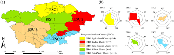
Figure 5. The spatial distributions of the 5 ES clusters (N represents the number of states); WY: water yield; HQ: habitat quality; FP: food production; SF: sand fixation; SR: soil retention; CS: carbon storage; and NPP: net primary production.
Download figure:
Standard image High-resolution imageAgricultural cluster (ESC 1): four states accounted for 15.96% of the study area and were mainly concentrated in Northern Kazakhstan (figure 5(a)), including North Kazakhstan, Akmola, Kostanay and Pavlodar. This cluster contains a high percentage (60.83%) of cropland (table 3), which provided higher provisioning services (FP) (figure 5(b)).
Table 3. The proportion (%) of land use/land cover types in each cluster.
| Forestland | Grassland | Cropland | Wetland | Urban | Bare land | Waterbodies | |
|---|---|---|---|---|---|---|---|
| ESC1 | 2.14 | 34.49 | 60.83 | 0.06 | 0.18 | 0.20 | 2.09 |
| ESC2 | 8.48 | 60.70 | 20.40 | 1.67 | 0.33 | 4.40 | 4.02 |
| ESC3 | 0.03 | 22.25 | 7.64 | 0.06 | 0.13 | 66.06 | 3.83 |
| ESC4 | 0.44 | 77.49 | 14.30 | 0.12 | 0.12 | 6.40 | 1.13 |
| ESC5 | 2.92 | 47.25 | 28.63 | 0.01 | 0.79 | 17.55 | 2.86 |
Carbon cluster (ESC 2): seven states accounted for 38.35% of the study area and were mainly distributed in eastern Kazakhstan and northwestern Kyrgyzstan, providing high CS (22.40%) and WY (15.70%) (figures 5(a) and (b)). The main vegetation types included grassland (60.70%) and farmland (20.40%) (table 3).
Sand fixation cluster (ESC 3): 11 states accounted for 28.35% of the study area and were mainly concentrated in southwest CA (figure 5(a)), such as Karakalpakistan, Kyzylorda, Dashgovuz, Lebap, and Navoiy. This cluster mainly comprised 66.06% desert or bare land with low vegetation coverage (table 3), providing high SF (32.01%) services (figure 5(b)).
Habitat cluster (ESC 4): six states accounted for 32.05% of the study area and mainly provided HQ (36.28%) and CS (18.57%) (figures 5(a) and (b)). This cluster was mainly concentrated in the central grassland of Kazakhstan, including Atyrau, Aktobe, West Kazakhstan, Karaganda, South Kaz and Zhambyl (figure 5(a)). Main vegetation types included grassland (77.49%) (table 3).
Soil and water cluster (ESC 5): 15 states accounted for 8.86% of the area of the study region and primarily included the southeastern mountain states (figure 5(a)). The land cover mainly comprised grassland (47.25%) and cropland (28.63%) (table 3). More rainfall and vegetation coverage could substantially promote SR (17.68%), WY (17.44%) and healthy ecosystem habitats (HQ: 26.38%) (figure 5(b)).
3.4. Interactions among ESs
A total of 21 potential trade-offs and synergies relationships between seven ESs were analyzed by Spearman's correlation coefficients at the ESC scales (figures 6(a)–(e)). For five different ESCs (figures 6(a)–(e)), SF displayed negative correlations with other ESs, especially in ESC1 (r = −0.34 to −0.66; p < 0.01) and ESC3 (r = −0.38 to −0.54; p < 0.01). FP was positively correlated (r = −0.2; p < 0.05) with NPP and SR in all ESCs (figures 6(a)–(e)). Good synergistic relationships existed pairwise between WY, SR, CS and NPP except for ESC3. Significant negative correlations (r = −0.21 to −0.66; p < 0.01 and p < 0.05) were found between FP and HQ in ESC1, ESC2 and ESC5 (figures 6(a), (b) and (e)), while a positive correlation (r = 0.39; p < 0.01) existed in ESC3 (figure 6(c)).
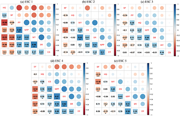
Figure 6. Correlation of paired ES under different ES clusters (ESCs) (**P < 0.01 and *P < 0.05; red color refers to trade off relationship, and blue color refers to present synergy relationship). WY: water yield; HQ: habitat quality; FP: food production; SF: sand fixation; SR: soil retention; CS: carbon storage; and NPP: net primary production.
Download figure:
Standard image High-resolution image3.5. Identification of driving factors among ES clusters
Sixteen driving factors affecting the spatial distribution of seven ESs were identified by a RDA in this study (figure 7). The explanatory variables of RDA account for 56.32%, 58.46%, 54.37%, 57.69% and 60.37% of the variation in ESC1, ESC2, ESC3, ESC4 and ESC5, respectively, indicating that the selected factors represented each ESC distribution well. Among all ESCs (figures 7(a)–(e)), PPT was positively correlated with WY, SR, CS and NPP; VC were positively correlated with SR, NPP and CS; S_d and TEM were positively correlated with SF; DEM, SL, PF and PG were closely related to HQ; and FP was explained more by PD, GDP, GD, PU and PC. Notably, trade-offs between socio-economic factors (e.g. PD, GDP, GD and PC) and HQ were found in figures 7(a), (b), (d) and (e).

Figure 7. Redundancy analysis of seven ESs (green color) and 16 socio-ecological drivers (red color) at the different ES clusters (ESC) scales. WY: water yield; HQ: habitat quality; FP: food production; SF: sand fixation; SR: soil retention; CS: carbon storage; and NPP: net primary production. PPT: annual total precipitation; TEM: annual mean temperature; VC: annual mean vegetation coverage; S_sand: soil sand content; S_clay: soil clay content; S_silt: soil silt content; S_c: soil organic matter content; DEM: digital elevation model; SL: slope; GDP: gross domestic product; PD: population density; and GD: grazing density; PC: percentage of cropland; PU: percentage of urban; PG: percentage of grassland; PF: percentage of forestland.
Download figure:
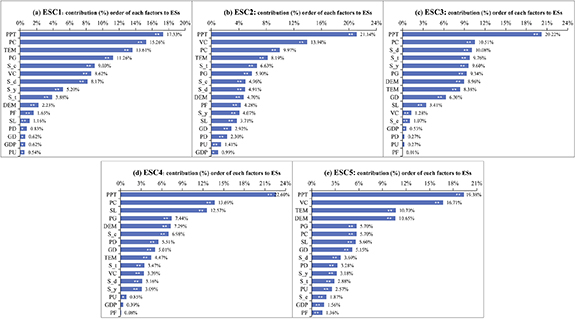
Standard image High-resolution imageMonte Carlo permutation tests were used to test whether the explanation of the ES distribution provided by the 16 environmental factors was significant. The factor contributions of the 16 factors presented differences throughout the ESCs (figures 8(a)–(e)). The spatial results of ESC1 (agricultural cluster) was dominated by provisioning services (FP) (figures 7(a) and 8(a)) and mainly determined by PPT (17.33%), PC (15.26%), TEM (13.61%) and PG (11.26%). ESC 2 (Carbon Cluster) (figures 7(b) and 8(b)), for which the importance of regulating services (CS) was high, was mainly affected by large values for PPT (21.14%) and VC (13.94%). PPT (20.22%) was still the most important driver of ESC3 (sand fixation cluster) distribution (figures 7(c) and 8(c)), followed by cropland (10.51%) and soil variables (9.60%–10.08%). In ESC4 (Habitat Cluster) (figures 7(d) and 8(d)), PPT (22.60%), PC (13.69%), SL (12.57%) and PG (7.44%) strongly impacted the multi-ESs. Figures 7(e) and 8(e) show that PPT, VC, TEM and DEM were the most important drivers affecting ESs for ESC5 (Soil and water cluster) with higher regulating services (SR and WY), accounting for 19.38%, 16.71%, 10.70% and 10.65% of the total explanatory variables, respectively. Notably, the explanatory power of PD, GDP and GD was low and not significant in 5 ESCs (figures 7(a)–(e) and 8(a)–(e)). By comparison, the contribution of the natural variables was much higher than that of the socio-economic variables, indicating that natural factors play a major role in the spatial distribution of ESCs (figures 7(a)–(e) and 8(a)–(e)).
Figure 8. Contribution order and significance test (**P < 0.01 and *P < 0.05) of 16 socio-ecological drivers in different ESCs scales. PPT: annual total precipitation; TEM: annual mean temperature; VC: annual mean vegetation coverage; S_sand: soil sand content; S_clay: soil clay content; S_silt: soil silt content; S_c: soil organic matter content; DEM: digital elevation model; SL: slope; GDP: gross domestic product; PD: population density; and GD: grazing density; PC: percentage of cropland; PU: percentage of urban; PG: percentage of grassland; PF: percentage of forestland.
Download figure:
Standard image High-resolution image
4. Discussion
Previous studies have indicated that the complex spatiotemporal patterns of ESs are caused by the highly heterogeneous terrain/landscape and complex socio-economic background in CA (Chen et al 2013, Li et al 2019a, 2020a). The conjoint analysis at ES clusters scale in this study further showed broad associations among ESs in CA (figures 6(a)–(e)), and revealed the complex controls of socio-ecological factors on the heterogeneous distribution of ES clusters in dryland (figures 7(a)–(e) and 8(a)–(e)). Identifying key socio-ecological variables and understanding how they co-vary to produce these consistent sets of ES are important to understanding the critical synergies and trade-offs between the complex landscapes in CA, such as mountain forests, river/riparian, irrigated cropland, grassland, and desert ecosystems (Spake et al 2017, Schmidt et al 2019, Schultner et al 2021).
4.1. Associations between ES clusters and socio-ecological driving factors
This study demonstrated that ES clusters in CA were much more sensitive to natural variables (e.g. climate and vegetation) than to socio-economic variables (e.g. population and economy) (figures 7(a)–(e) and 8(a)–(e)). Previous studies have indicated that stressed ecosystems like dryland are mainly controlled by natural environment factors (Chen et al 2019a, Zhu et al 2019, Li et al 2021). Among the environmental variables, we found that PPT and VC were the main factors influencing the associations among ESs (figures 8(a)–(e)). PPT (17.33%–22.60%) was the most important driver for promoting positive correlation between the WY, SR, CS and NPP services (figures 7(a)–(e) and 8(a)–(e)). The increase in rainfall directly changes surface runoff and detaches soil particles, indirectly leading to the increase in water production and soil water erosion (Ran et al 2012, Fang et al 2015). Furthermore, PPT has been proved to be the dominant factor regulating carbon stocks of dryland in CA (Zhu et al 2019). The ephemeral plants determine approximately 75% of the water/carbon and biomass dynamics in the temperate desert communities (Gang and Li 2014), and their biomass is closely correlated with the rainfall fluctuations during the growing season (Wang et al 2006). With a 0.4 °C decade−1 warming rate during the past 30 years, CA is a hotspot of climate change (Hu et al 2014). Considering the high sensitivities of ES clusters to climate change and the high uncertainties of future climate trajectories in this region (Thevs et al 2013, Han et al 2016, Li et al 2020a), it is advisable for policymakers to closely monitor climate change patterns and prepare adaptive ecological management strategies (e.g. limiting irrigation water usage and reducing grazing stress to protect VC in the ESC2 and ESC5 which were most sensitive to PPT) in advance based on future climate scenarios (figures 8(b) and (e), Saidi and Spray 2018, Schierhorn et al 2020). When PPT was not a limitation factor, we found that the synergies among SR, NPP and CS among ES clusters were closed related to VC (figures 7(a)–(e)), especially in the mountain cluster (ESC5) (figure 8(e)). This finding is consistent with a previous research (Zhang et al 2020a), and is reasonable because VC is a good indicator of soil erosion, carbon sequestration, ecosystem productivity, etc (Chaitra et al 2018, Deng et al 2021).
Overall, our results are similar to other studies in arid regions (Lyu et al 2019, Dou et al 2020). Although the explanatory power of some socio-economic factors (e.g. PD, GDP and GD) was low in CA (figures 8(a)–(e)), the antagonistic effects of these factors on HQ cannot be ignored in cross-regional ecological management (figures 7(a)–(e), Sallustio et al 2017). Good habitat environment was provided by large areas of grassland (77.49%) to maintain the biodiversity in habitat cluster (ESC4) (figure 5(b) and table 3). This area has been listed as a key biodiversity protection area by international organizations (Wagner et al 2020). Nature reserves and ecological corridors should be established to effectively reduce intensive grazing activities and raise the species protection awareness of the local population (Liu et al 2009, Negev et al 2019).
4.2. Following the ES clusters to guide ecological management
An important recommendation provided by this study is that ES clusters (rather than administrative or land-cover/land-use boundaries) should be treated as the basic ecological management unit in CA (Spake et al 2017), and different management strategies should be designed in accordance to the major interactions among the ESs in each ES cluster (Chen et al 2020). For example, an obvious negative relationship between high provisioning services (FP) and regulating and maintenance services (HQ) was found in ESC1 (figures 5(b) and 6(a)), which indicates that it is necessary to balance the trade-off between FP and HQ to promote the overall ESs in this region (Bernués et al 2019). Land management activities (like converting ecological land to cropland) that enhance certain ES (e.g. FP) at large costs to other ESs should be prevented (Searchinger et al 2015). In contrast, good synergies among CS and other regulating services were found in ESC2 (figures 5(b) and 6(b)). Measures such as increasing vegetation coverage and forestland area should be taken to stabilize the synergies between these ESs (figures 7(b) and 8(b), Mouchet et al 2017, Zhang et al 2020a).
However, effective ecological management policies based on ES clusters would require cross-country coordination (Kumar 2002, Batsaikhan and Dabrowski 2017). Since 2000, with the assistance of the United Nations and other regional organizations (Mangalagiu et al 2019), policies and laws on ecological protection, such as the Implementation of integrated water resource management (UNDP 2004), the Implementation of Integrated Pollution Prevention and Control (IPPC) (UNECE 2010), Law on Environmental Protection (Hao et al 2019), etc, have been continuously stipulating and integrating into international practices. Under the coordination of UNDP and UNECE, the five CA countries have made great progress in ecological protection in recent years (Suleimenov et al 2012, Turayeva 2012, Thevs et al 2013), but different attitudes towards ES management have created challenges to the Sustainable Development Goals. One of the challenges is how to balance the short-term and local ES benefits with the long-term and global ES values (Milner-Gulland 2012, McPhearson et al 2013). For example, promoting FP through farmland expansion is attractive to CA countries because it brings quick and materialized benefits to local societies (Schierhorn et al 2020). However, farmland expansion would also lead to degradation of other continental or globally important ESs (Li et al 2015, 2020a), such as SF (CA is the major sand-dust source to the northeastern Asia) and HQ (CA accounts for over 80% of global temperate desert ecosystems).
Therefore, cross-ES clusters coordination is important for understanding the associations among ESs and managing regional ES as an integrated system (Malmborg et al 2021). For example, although the ESC5 was mostly distributed in the mountainous areas (figures 1(a) and 5(a)) with low PD and economic development level, its water resources were the cornerstone of the normal supply of ESs in the sand fixation cluster (ESC3) (figure 5(b), Hao et al 2019). Also, the regulating services (e.g. WY and SR) from the upstream cluster (ESC5) had regional importance to other ES clusters (figures 1(a) and 5(a), Li et al 2021). To avoid losing the erosion regulating service and promote sustainable soil management (Jin et al 2008), deforestation should be banned and cropland on steep slopes should be converted into forestland in these areas (Decocq et al 2016, Eguiguren et al 2019). However, the value of regulating services not reflected in economic markets (Raudsepp-Hearne et al 2010). For all clusters, policy makers should prioritize implementing a series of compensation for ES (PES) policies (Fu et al 2018, Lin et al 2020), including 'Conversion of Farmland to Forests Compensation' (Yang et al 2019) and 'Returning Grazing Land to Grassland (Shao et al 2016),' to reduce the economic losses of residents through government subsidies (McElwee et al 2020).
5. Conclusions
Advancing the ES clusters approach, we proposed a new framework for identifying the relative importance of socio-ecological drivers that affect the ES clusters. The ES quantification indicated the spatial segregation and concordance of different types of ESs. Five types of clusters were identified in this study, including the 'agricultural cluster' (ESC1), 'carbon cluster' (ESC2), 'sand fixation cluster' (ESC3), 'habitat cluster' (ESC4) and 'Soil and water cluster' (ESC5). Similarities and differences of the synergies and trade-offs between ESs existed in different ES clusters. The RDA analysis showed that the contribution of ecological variables (e.g. climate and vegetation) to the distribution of ES clusters was much higher than that of socio-economic variables (e.g. population and economy). Importantly, our study contributed a reproducible assessment framework that can be used for spatially target decision-making rated to ES. Nevertheless, some limitations still exist in this research. Lack of data is often regarded as a barrier to achieving comprehensive ES assessment. Our study were not able to access sufficient data on cultural values to include cultural ESs in our analysis, but we hope at a later stage to achieve this using questionnaires, observation, literature and public participation. In addition, we only used correlation analysis to explore linear relationship among ESs, we also hope further reveal non-linear characteristics between ESs using multiple regression analysis and least-square methods.
Acknowledgments
We thank the reviewers for their constructive comments that greatly helped us to improve the quality of this manuscript. This project was funded by the Strategic Priority Research Program of the Chinese Academy of Sciences (Grant No. XDA2006030201) and the State Key Laboratory of Desert and Oasis Ecology (#Y471163). Chi Zhang is supported by the Taishan Scholars Program of Shandong, China (Grant No. ts201712071).
Data availability statement
The data generated and/or analysed during the current study are not publicly available for legal/ethical reasons but are available from the corresponding author on reasonable request.