

Abstract
Arctic surface temperature has increased at approximately twice the global rate over the past few decades and is also projected to warm most in the 21st century. However, the mechanism of Arctic vegetation response to this warming remains largely uncertain. Here, we analyse variations in the seasonal profiles of MODerate resolution Imaging Spectroradiometer Leaf Area Index (LAI) and ERA-interim cumulative near-Surface Air Temperature (SATΣ) over the northern Russia, north of 60° N for 2000–2019. We find that commonly used broad temporal interval (seasonal) trends cannot fully represent complex interannual variations of the LAI profile over the growing season. A sequence of narrow temporal interval (weekly) LAI trends form an inverted S-shape over the course of the growing season with enhanced green-up and senescence, but balanced during the growing season's peak. Spatial patterns of weekly LAI trends match with those of weekly SATΣ trends during the green-up, while the drivers of the browning trends during senescence remain unclear. Geographically the area with the statistically significant temperature-driven enhanced green-up is restricted by a large patch carrying significant positive SATΣ trends, which includes North Siberian Lowland, Taimyr, Yamal and adjacent territories. The strength, duration and timing of the changes depend on vegetation type: enhanced green-up is most pronounced in tundra, while enhanced senescence is pronounced in forests. Continued release of the climatic constraints will likely increase the capacity both of the environment (i.e. permafrost thawing) and vegetation (i.e. appearance of more productive woody species), and transform LAI seasonal shifts to change of LAI seasonal amplitude.
Export citation and abstract BibTeX RIS

Original content from this work may be used under the terms of the Creative Commons Attribution 4.0 license. Any further distribution of this work must maintain attribution to the author(s) and the title of the work, journal citation and DOI.
1. Introduction
The 'greening trend', an increase of green biomass in response to the warming at northern high latitudes (north of 40° N) over the past 40 years, has been analysed in many studies at global and regional scales. Using time series of Vegetation Indices (VIs) derived from the NOAA Advanced Very High Resolution Radiometer (AVHRR) and NASA MODerate resolution Imaging Spectroradiometer (MODIS) data sets, a strong greening trend has been detected in the boreal zone, especially across Eurasia in the first half of the records (Myneni et al 1997, Zhou et al 2001, Nemani et al 2003, Stow et al 2004, Goetz et al 2005). However, in the 21st century the trend has substantially diminished: the rate of the amplitude increase has lowered and changes have mostly focused on seasonal shifts, the spatial pattern of greening has become fragmented and vegetation changes over the Arctic have become distinctive among those in the northern high latitudes (Zeng et al 2011, 2013, Xu et al 2013, Wang et al 2015, Zhao et al 2015, Park et al 2016, Zhu et al 2016, Elsakov 2017, Berner et al 2020).
According to the latest IPCC (www.ipcc.ch/site/assets/uploads/2017/09/WG1AR5_Frontmatter_FINAL.pdf) and NOAA (www.arctic.noaa.gov/Report-Card) reports, Arctic surface temperature has increased at approximately twice the global rate over the past few decades (the 'Arctic amplification' effect) and the region is also projected to warm most in the 21st century. Recent simulations with ecological niche and process-based models have predicted that under continued warming 10%–50% of vegetated areas of the Arctic may increase fractional cover and/or shift to a different physiognomic class with a dominance of woody cover by the 2050s (Kaplan et al 2003, Cheaib et al 2012, Macias-Fauria et al 2012, Kravtsova and Loshkareva 2013, Pearson et al 2013, Myers-Smith et al 2015, Rees et al 2020), through so-called 'tundra shrubification' (Park et al 2016) and 'forest advance' (Rees et al 2020) mechanisms, according to the hypothesis of 'easing climatic constraints' on vegetation development, especially temperature, but also radiation and precipitation in case of the Arctic (Nemani et al 2003, Keenan and Riley 2018, Rees et al 2020). Long-term field surveys, dendroecological analysis and high-resolution remote sensing generally corroborate these changes in Arctic vegetation (Kharuk et al 2006, Elsakov and Kulyugina 2014, Forbes et al 2014, Frost and Epstein 2014, Matveeva et al 2014, Rees et al 2020, Tishkov et al 2020). However, confirmation at the regional to global scale will require estimates based on moderate-resolution remote sensing data and these remain largely uncertain. These uncertainties arise because the solution of the complex monitoring task (i.e. due to persistent cloudiness, short growing season, sparse vegetation vulnerable to rapidly changing weather) (Stow et al 2004, Wang et al 2018) is attempted in terms of standard data processing and analysis techniques (i.e. the use of radiometric proxies for biophysical parameters, broad temporal interval (seasonal) averages and spatial aggregation), significantly limiting potential of modern remote sensing data sets (Berner et al 2020, Myers-Smith et al 2020).
This paper aims to advance our understanding of the mechanism of vegetation greenness changes over northern Russia in the 21st century. Specifically, we (a) accurately quantify interannual changes in the entire seasonal profile of vegetation greenness based on the past 20 years (2000–2019) of a weekly 230 m MODIS Leaf Area Index (LAI) product, and (b) attribute the observed changes in terms of climate forcing based on ERA-Interim reanalysis near-surface air temperature (SAT) data. Our analysis relies on the implementation of the following enhancements to the standard data processing methodology: (a) radiometric parameters (VI) are replaced with biophysical parameters (LAI) to directly quantify green foliage amount, (b) seasonal LAI averages are replaced with a weekly LAI profile to fully capture seasonal dynamics, (c) seasonal temperature averages are replaced with a weekly profile of cumulative temperature to quantify the actual biological forcing of foliage development (Nemani et al 2003, Hope et al 2005, Walker et al 2012, Shen and Cong 2015, Zhu et al 2016, Keenan and Riley 2018). Here we focus on the role of cumulative temperature; the potential impacts of other drivers, such as radiation and precipitation, as well as change in the environment (sea-ice and permafrost) are not considered independently in the study.
2. Data and methods
The vegetated land of Russia, north of 60° N is analysed in this study. The focus of this paper is on the Russian Arctic, which we define as the area within the Arctic Circle (north of ∼65° N), where most of climate related changes in vegetation greenness have been detected. More southerly areas often exhibit non-climate related vegetation regrowth after disturbances and were analysed to contrast both mechanisms of greenness change. According to the Space Research Institute of the Russian Academy of Sciences (hereinafter IKI) landcover map (figure 1) the territory is covered by boreal forests (52%), tundra (30%) and other vegetation, such as peatland, riparian vegetation etc (18%). We provide a separate analysis for tundra and forest, as these landcover categories exhibit significantly different sensitivity to climate variations (Beck and Goetz 2011, Bi et al 2013, Park et al 2016). We emphasize the tundra-forest ecotone as this transition zone is most sensitive to changing climate (Cheaib et al 2012, Berner et al 2013, Rees et al 2020). Due to the diverse terrain forms and climatic conditions of the territory (https://en.wikipedia.org/wiki/Great_Russian_Regions) we further split the analysis by regions (figure 1): West Siberian Plain (WSP), North Siberian Lowland (NSL), Central Siberian Plateau (CSP), Yamal (YML), Taimyr (TMR).
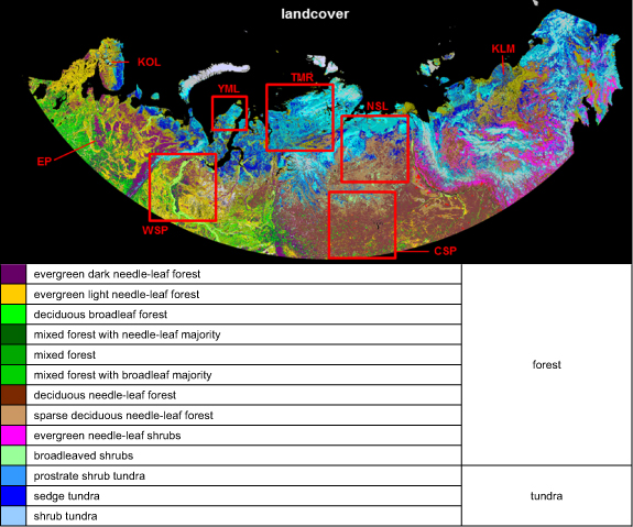
Figure 1. Study area- vegetated land of Russia, north of 60° N. Vegetation types in the area are characterised by the 23 class IKI landcover map (product for year 2010 is shown, Albers projection at 230 m). Classes were further aggregated into forest (52% of all land pixels), tundra (30%) and other categories. Frames indicate study sub-regions selected for further analysis based on different regimes of climate-vegetation interactions: West Siberian Plain (WSP), North Siberian Lowland (NSL), Central Siberian Plateau (CSP), Yamal Peninsula (YML) and Taimyr Peninsula (TMR). Also marked are territories mentioned in the text: European Plain (EP), Kola Peninsula (KOL) and Kolyma (KLM).
Download figure:
Standard image High-resolution image2.1. Satellite data sets
In this study vegetation is characterized by the MODIS LAI and landcover remote sensing products developed at IKI, while climate forcing is represented by the near-SAT fields from the European Center for Medium Range Weather Forecast (ECMWF) Interim reanalysis product (ERA-Interim).
The IKI products are generated within the data management and processing facility, which routinely downloads NASA MODIS Aqua and Terra surface reflectance products (Collection 6), applies pre-processing (cloud/snow masking and compositing) and higher level (including landcover, Normalized Difference Vegetation Index (NDVI), LAI, etc) algorithms to generate time series of advanced accuracy products for monitoring the natural resources of Russia. The IKI MODIS landcover is an annual product (from 2000 to present) at 230 m resolution, with 23 classes (those relevant to this study are shown in figure 1). The classification algorithm is a maximum likelihood implemented within the Locally Adaptive Global Mapping Algorithm (LAGMA) classifier (Bartalev et al 2014).
The IKI MODIS LAI is a cloud- and snow-screened weekly composited and interpolated product at 230 m resolution, over the period from April 2000 to the present. The daily LAI retrieval algorithm is an enhanced version of the NASA MODIS Collection 6 algorithm (https://lpdaac.usgs.gov/documents/624/MOD15_User_Guide_V6.pdf). This is a radiative transfer (RT) based approach, where LAI retrievals are performed based on the Red and NIR channel data (Knyazikhin et al 1998). RT simulations were re-generated at IKI based on the latest advances in stochastic RT modelling to characterize canopy structure (Huang et al 2008, Shabanov and Gastellu-Etchegorry 2018). We also extended the dynamic range of Solar Zenith Angle (SZA) up to 70° (with a step of 5°) for more accurate retrievals at high latitudes (Stow et al 2004). Daily retrievals are cloud- and snow-filtered using a statistically based IKI mask (Bartalev et al 2016). Cloud/snow masking is especially challenging in the Arctic because (a) cloud cover is highly variable and depends on changing sea-ice coverage in the coastal zone, (b) cloud shadows are especially strong (due to high SZA), (c) residual snow cover may be patchy and mixed with the vegetation signal (Wang et al 2018, Myers-Smith et al 2020). Additional screening was applied to filter stripes appearing in MODIS Red channel at low red and high SZA values: data with Red<0.02 and SZA> 60° were screened out. At the next step, weekly compositing is applied to the retained data to select the median value. Compositing is performed on a fixed temporal grid, starting from 1 January. Compositing dates are referred to by the starting date. At the next step temporal interpolation is performed using the Locally Estimated Scatterplot Smoothing (LOESS) method implemented with second-order polynomials and a sliding window approach (Plotnikov et al 2014). This helps to suppress noise, fill gaps, but still preserving local data variability. The IKI MODIS LAI product inherits its maturity status from the corresponding NASA product, which has been widely used in applications over the past two decades (Yan et al 2020), validated globally (i.e. Yang et al 2006) and intercompared with key peer products (i.e. Garrigues et al 2007). The accuracy of the former should therefore be at least equal to that of the latter, i.e. 20% (Yang et al 2006). A recent validation study of the IKI MODIS LAI product over sparse boreal forests of Kola Peninsula (KOL) reported an accuracy of ∼7.5% (Shabanov et al 2021).
ERA-interim gridded near-SAT was obtained from the ECMWF Interim Reanalysis (Dee et al 2011) at six-hourly intervals (0, 6, 12, 18 UTC) at a spatial resolution of 0.7° (∼75 km) over the period from March 2000 till August 2019. This product was selected from alternatives (including the newer ECMWF ERA5 reanalysis) as it has the smallest overall errors in SAT across Arctic Russia, based on a validation against observations from 67 meteorological stations (internal testing). Due to the large east–west extent of Russia, a daily averaging procedure was implemented to avoid the impact of the diurnal cycle. As vegetation greenness is most sensitive to cumulative rather than instantaneous temperature, we performed accumulation of average daily temperature starting from 1 March until the end day of the corresponding LAI compositing period, provided that the average temperature exceeded a +5 °C threshold. This variable is referred hereafter as SATΣ.
All data were resampled to a common grid, based on the Albers projection at 230 m spatial resolution, covering Northern Russia, north of 60° N.
2.2. Methodology
The use of radiometric quantities (VIs) and long period (growing season or seasonal) temporal averages was appropriate for limited accuracy NOAA AVHRR time series data. In this analysis we have attempted to fully utilise the potential of the time series of the LAI biophysical parameter derived from the NASA MODIS data (i.e. excellent orbit stability, geolocation and radiometric accuracy, availability of atmospheric correction, etc) using advanced data pre-processing techniques. This level of data accuracy made possible to avoid temporal averaging and work with the seasonal LAI profile directly. To characterise changes of greenness we implemented least-squares linear regression of the seasonal LAI profile for each weekly period (up to 52 regressions/year).
In this research we did not follow standard approaches to quantify the (change of) phenology, based on fitting a sigmoid curve. According to a recent studies (Zhang et al 2017, Wang et al 2018) the standard methodology faces the following issues over the pan-arctic regions: (a) growing season duration is very short, and curve fitting is challenging due to limited data availability because of snow and/or cloud contamination, (b) estimates of start-of-season and end-of-season dates are often affected by snow, (c) LAI-like indices perform better than commonly used VIs. In this study we refrain from quantifying phenology shifts in terms of 'number of days of spring/fall advance', as the change of greenness depends on date, so that effectively this means that the 'advance' varies with the date. The seasonal profile of change provides more detailed information.
To quantify the potential impact of climate change on LAI time series we avoided using seasonal averages of temperature, and utilized cumulative near-SAT (SATΣ) instead. That is, we view vegetation as a system with memory, the current condition of which depends on the thermal history. Sensitivity tests indicate that during the green-up period cumulative temperature is best correlated with LAI. However, after transitioning into the senescence phase this correlation steadily diminishes, and even becomes negative.
To ensure the stability of the results of statistical analysis (especially trends), time series for each pixel were further filtered to retain only those, for which at least six valid values per length of time series were available. Ordinary least square method was used to calculate trends in time series of LAI and SATΣ. The parametric Student's t-test was utilized to assess the significance of trends using threshold p < 0.1, a Gaussian noise model was assumed and an autocorrelation test was applied. While the autocorrelation test for LAI may be optional for the sparse vegetation vulnerable to rapidly changing weather in the Far North, it is required for dense stable forests in the Southern part of the study area. Likewise, the autocorrelation test may have a minor impact on screening cumulative temperature trends at the beginning of the growing season (due to random daily weather variations), but autocorrelation may significantly increase at the end of the growing season, as daily weather variations are suppressed through data accumulation over a repeated annual cycle. To apply this methodology uniformly, we used the autocorrelation test for both variables through the whole growing season. The Pearson correlation coefficient was implemented to evaluate correlation, along with the Student's t-test to assess its significance. The assumptions and sensitivity tests are essentially the same as for the trend analysis.
Trends in this paper are presented as relative quantities, as severity of changes is quantified by a deviation from the normally expected value, ΔLAI = (LAI end − LAI start )/LAI mean , where all quantities are derived from the regression analysis, LAI start corresponds to the regression estimate for the start of period (2000), LAI end for the end of period (2019), and LAI mean is the mean value between the two endpoints. In this paper we refer to positive trends of ΔLAI as 'greening' and negative trend as 'browning', following the remote sensing terminology (Myers-Smith et al 2020). However, we emphasise that the retrieved trends may be affected by concentrations of leaf chemical constituents (e.g. chlorophyll content), as these are not decoupled from the green foliage amount in the current parameterization of the LAI algorithm. Likewise ΔSATΣ is similarly defined to ΔLAI. This way trends can be comparable across the dynamic range of LAI and SATΣ over diverse environmental conditions. Numerically this results in a better localisation (smaller dynamic range) of peaks of most typical values.
3. Results and discussion
3.1. Maximum LAI analysis over the whole study area
To establish a baseline for the new methodology we performed a standard trend analysis based on the seasonal maximum LAI data set (hereinafter LAI max ) (figure 2). The day when LAI max is reached in the study area may vary by ± two weeks but is typically observed on day 195 (July 13), with forest earlier (193), and tundra later (200), primarily due to the negative south–north temperature gradients (figure 2(iii)). LAI max varies substantially with vegetation type: tundra between 1 and 2 (mean 1.8) and forest between 1 and 6 (mean 3.2) (figure 2(iv)). However, there are no distinct changes in LAI max when crossing the ecotone from (sparse) forest to tundra (cf figures 1 and 2(i)). We also note that there is no spatial coherence between variations of landcover, LAI max and relative LAI max change (hereinafter ΔLAI max , cf figure 2(ii)). The histogram of ΔLAI max over all vegetation is centred on close to zero changes (−0.2%) over the past 20 years, with tundra slightly greening (+1.5%) and forest slightly browning (−0.5%) (figure 2(v)). Overall balance is a counter-balancing effect of positive/negative changes of a moderate magnitude (STD ∼ 20%). The largest contiguous areas showing positive trends are observed in the far-northern territories of YML, TMR and the eastern part of NSL and some fragmented regions in the far-east. The trends with the largest amplitude are observed in Central Siberia, being both negative and positive, caused by fresh disturbances (fire/clear-cuts, distinguishable by the regular shape of patches) and subsequent regrowth of vegetation. Seasonal summer (JJA) average LAI time series (not shown) indicate similar spatial distribution to LAI max (figure 2(i)). The reason for this is discussed in the next section. We note that the spatial distribution of LAI max trends in this study is consistent with those obtained using the NASA MODIS NDVI product for 2000–2016 (Elsakov 2017). We also note that the highly fragmented spatial distribution of ΔLAI max is inconsistent with macro-scale patterns of atmospheric forcing (cf next section), therefore a correlation analysis between ΔLAI max and temperature was not performed.

Figure 2. Seasonal maximum LAI analysis over the whole study area. Top panels show maps of average (<LAI max >) and relative change (ΔLAI max ) of seasonal maximum LAI over period 2000–2019 (Albers projection at 230 m). Lower panels demonstrate key statistics of LAI max data set, split by vegetation type (tundra and forest): distributions of average dates when LAI max is achieved, LAI max , and ΔLAI max .
Download figure:
Standard image High-resolution image3.2. Seasonal LAI and SAT∑ profile analysis over the whole study area
In this section we extend the foregoing analysis from a single time series of seasonal LAI max to a set of weekly LAI time series over the course of the seasonal profile. This type of analysis allows us to trace the association between the time series of LAI and SATΣ in terms of correlation between two variables. Figure 3 shows maps of seasonal trends ΔLAI and ΔSATΣ, and also corr(LAI, SATΣ) (cf section 2 for definition) for compositing dates 148 (∼27 May), 169 (∼17 June), 197 (∼15 July) and 225 (∼12 Aug), representing different phases in the seasonal dynamics of each data set. The sequence of ΔLAI maps (figure 3(i)) demonstrates that large-scale spatially homogeneous patterns of greening/browning exist and their amplitude and location transform over the course of the growing season. For date 148, large homogeneous patterns of greening affect the European Plain (EP), KOL and CSP, while WSP exhibits browning. By date 169 the strong greening in EP has subsided, the conditions of WSP and CSP remain essentially unchanged, but very strong greening affects NSL. By mid-summer (day 197), the greening has moved further north and affects mostly YML, TMR and the northern part of NSL, while EP and WSP exhibit a mix of greening and browning patches, while CSP remains unchanged. Finally, toward the fall, NSL and CSP exhibit strong homogeneous patterns of browning, while YML and TMR show greening. Thus, over this three-month period the Russian Arctic exhibits significant spatial and temporal variability of greening and browning. The spatial distribution of trends of LAI max (figure 2(ii)) is most similar to seasonal trends for compositing period 197 (figure 3) because the maximum typically occurs at date 195 (figure 2(iii)).
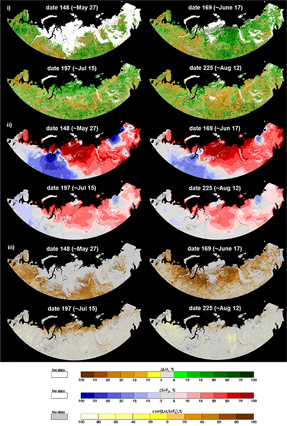
Figure 3. Seasonal LAI/SATΣ profile analysis over the whole study area—dynamics of spatial distribution. Panel (i): sequence of maps showing relative change of leaf area (ΔLAI) at different phases in the seasonal dynamics. Panel (ii): the same but for relative change of cumulative temperature (ΔSATΣ). Panel (iii): the same but for correlation of LAI and SATΣ. Correlation data are screened to retain significant values at p < 0.1. Maps are presented in the Albers projection at 230 m.
Download figure:
Standard image High-resolution imageThe observed changes in the patterns of ΔLAI (greening/browning) during the green-up phase match the corresponding spatial patterns of ΔSATΣ (figure 3(ii)). The strongest warming forcing is primarily observed in the far-northern territories, NSL, TMR, YML and adjacent territories, while cooling is focused in WSP and Kolyma (KLM). Also note that the far-eastern territories of northern Russia have experienced a relatively moderate increase of SATΣ during the snow-free period, resulting in limited (and spatially fragmented) increase of leaf area. The strength of association between temperature forcing and vegetation response reaches its maximum during the green-up phase (dates 148–169), as can be seen by cross-comparing patterns of the spatial consistency of warming/cooling forcing (ΔSATΣ) and greening/browning response (ΔLAI). However, as vegetation reaches its maximum development by mid-summer (date 197) the correlation between SATΣ and LAI ceases and strong negative ΔLAI trends during the senescence phase (date 225) remain unattributed (cf figure 3(iii)). Also, comparing the maps of landcover (figure 1) and correlation (figure 3(iii)), it is apparent that during the course of the year, the pattern of significant correlation crosses the forest-tundra ecotone and remains persistent over regions of tundra rather than forest (as especially noticeable in the correlation map for date 197).
Changes in the seasonal dynamics of LAI under the influence of changes in SATΣ are numerically quantified in figure 4. Analyses are performed separately for tundra and forest, and all vegetated areas combined together. The top row (figures 4(i)-(iii)) shows the seasonal variation of LAI and ΔLAI, averaged over their respective distributions (i.e. similar to figures 2(iv)–(v) for LAI max ). In general, for both vegetation types the changes form an inverted S-shape over the course of the growing season: (a) enhanced non-monotonic greening during green-up (up to 18% for tundra), (b) enhanced monotonic browning during senescence (up to −15% for forest), and (c) balanced at the seasonal peak. The most interesting aspect of the balance between greening and browning is that LAI and its change are in 'opposite phases': when LAI reaches its maximum the changes are close to zero. Furthermore, since enhanced greening and enhanced browning are approximately balanced, trends calculated from summer season (JJA) averages are also close to zero. Our results are generally consistent with those shown in Park et al (2016), which reports an advance of both the start and end of the growing season in Arctic Eurasia, based on analysis of AVHRR NDVI time series 2000–2014.
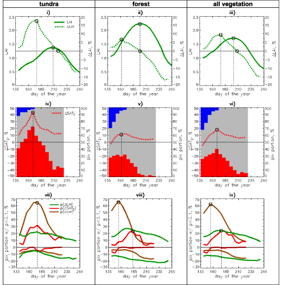
Figure 4. Seasonal LAI/SATΣ profile analysis over the whole study area—dynamics of statistics. Top row: seasonal variations of mean leaf area and its mean relative change (ΔLAI) for tundra, forest and all vegetation together. Middle row: seasonal variations of mean relative change of cumulative temperature (ΔSATΣ). In the background are shown seasonal variations of percentage of pixels with positive (red), negative (blue) and neutral (grey) trends of SAT∑. Bottom row: seasonal variations of portions of pixels with significant (p < 0.1) trends of LAI, SATΣ and significant corr(LAI, SATΣ). Positive (negative) branches correspond to amounts with positive (negative) trends or correlation.
Download figure:
Standard image High-resolution imageThe seasonal course of ΔSATΣ is shown in the middle row of figure 4. Additionally presented are the proportions of pixels falling into three categories: strong negative trends with relative changes in the range (−100%, −20%), neutral (−20%, +20%) and strong positive changes (+20%, +100%). From figures 3 and 4 (middle row) it can be inferred that tundra has experienced the strongest warming forcing (YML, TMR and NSL), while the warming forcing in forested regions was more modest and uniform over time (EP, CSP), and for some areas (WSP) cooling was experienced. The timing of the maximum ΔLAI matches that of maximum forcing (ΔSATΣ) for both vegetation types (dates 169–176), but the strength of increase is very different: sharp peaks of both variables are observed for tundra, but this feature is supressed for forests. Further details on the strength of association between SATΣ and LAI seasonal trends can be obtained by intercomparing seasonal profiles of portion of pixels with significant trend and significant correlation between the two variables as shown in figure 4 (last row). For tundra all three variables are in phase, and this effect can be interpreted as climate-driven greening. However for forests the phases of the three variables do not match. Namely, according to the seasonal profile of corr(LAI, SATΣ), the ΔSATΣ drives the ΔLAI only early in the growing season, while major portion of significant ΔSATΣ appear later in the season. The nature of this effect is best understood at the level of regional subset analysis (cf the next section). In addition to the seasonality of greening trends, consider the seasonality of browning trends: the portion of pixels with significant negative ΔLAI increases toward the end of the growing season and the effect is much more pronounced for forest. As the significant SATΣ trends are almost always positive, they cannot explain the negative LAI trends.
Finally, note that a similar approach, to trace the variation of the entire seasonal profile of AVHRR NDVI (instead of maximum NDVI) and surface temperature has been implemented recently for the whole panarctic tundra over the period 1999–2015 (Bhatt et al 2017). The results of that study, namely an early spring NDVI decline and increase of surface temperature, are inconsistent with our findings and with those of Park et al (2016), but this could be due to differences in methodologies and data sets (Myers-Smith et al 2020). The results of trend analysis are highly sensitive to accuracy of data, and while the MODIS data with advanced pre-processing may be suitable for the seasonal profile analysis, the AVHRR data may still best be analysed with the standard methodologies involving spatial and temporal averaging.
3.3. Seasonal LAI and SAT∑ profile analysis over the regional subsets
Both climate forcing and the response of vegetation vary across different regions of the northern Russia. The results of our analysis over the regional subsets (cf figure 1) are presented in figures 5–7. More details are presented for the NSL and CSP subsets in order to contrast changes between tundra and forest and also the tundra-forest ecotone.

Figure 5. Seasonal LAI/SATΣ profile analysis over the NSL subset featuring tundra-forest ecotone. Panels (i)–(iv) show map of LC for year 2010 and also maps of ΔLAI, LAI start LAI end for date 169, when maximum correlation between LAI and SATΣ is achieved. Panels (v)–(vi) show sequence (for dates 155–225) of ΔLAI and corr(LAI, SATΣ) maps screened to retain significant trends/correlation (p < 0.1) to highlight different temporal phases of LAI changes and it association with SATΣ changes. Color tables for maps are shown in figures 1–3. Panel (vii) shows seasonal variation of mean over subset values of LAI, ΔLAI, ΔSATΣ and corr(LAI, SATΣ). Panel (viii) demonstrates coherence of subset-averaged values of LAI and SATΣ over the course of time series for the date of maximum correlation. Values d(LAI) and d(SATΣ) denote regression based absolute changes of corresponding variables over the course of time series. Panel (ix) shows seasonal variations of portions of pixels with significant (p < 0.1) trends of LAI, SATΣ and significant corr(LAI, SATΣ). Positive (negative) branches correspond to amounts with positive (negative) trends or correlation.
Download figure:
Standard image High-resolution image
Figure 6. Seasonal LAI/SATΣ profile analysis over the CSP subset occupied by dense forest under disturbances (fires and clear-cuts). The same type of results is shown as in figure 5 for the NSL region. In case of the SCP region maximum correlation is achieved at date 148.
Download figure:
Standard image High-resolution image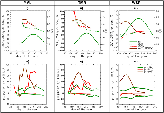
Figure 7. Seasonal LAI/SATΣ profile analysis over the other subsets of interests: YML(tundra), TMR (tundra) and WSP (broadleaf forest). Top row: seasonal variation of mean over subset values of LAI, ΔLAI, ΔSATΣ and corr(LAI, SATΣ). Bottom row: seasonal variations of portions of pixels with significant (p < 0.1) values of ΔLAI, ΔSATΣ and corr(LAI, SATΣ).
Download figure:
Standard image High-resolution image
3.3.1. NSL
Figure 5 presents the results of analysis over the NSL subset. According to the landcover map (figure 5(i)), this area is a transition from deciduous needle-leaf forest (53%, mostly sparse Larix) in the south to tundra (32%, mostly shrubland) further north. Figures 5(ii)–(iv) show maps of ΔLAI, LAI start and LAI end for date 169 when maximum ΔLAI is achieved. The latter two variables are regression-based LAI estimates for the first (2000) and the last (2019) years of the time series, respectively. Comparing LAI start and LAI end greenness appears to expand from forest to tundra (consistent with the 'tundra shrubification' scenario (Park et al 2016)). Figures 5(v) and (vi) present a sequence over time of ΔLAI and corr(LAI, SATΣ) maps, screened to retain significant values, p < 0.1, to highlight different temporal phases of corresponding variables. In the above sequences observe the following: (a) the steady replacement of positive ΔLAI trends (greening) at the beginning of time series with negative ones (browning) toward the end of series, (b) phases of ΔLAI and corr(LAI, SATΣ) match, an indicator of climate-driven changes of greenness, (c) both tundra and forest are exposed to a common pattern of strong warming (figure 3(ii)), but their response is different: tundra exhibits a stronger and more temporary persistent association between LAI and SATΣ, while more forest pixels have significant LAI trends.
Consider results of numerical analysis of seasonal variations of LAI, ΔLAI, ΔSATΣ and corr(LAI, SATΣ) for all vegetation types together as shown in figures 5(vii)–(ix). According to figure 5(vii) vegetation is sparse (LAI max ∼ 1.5), but seasonal LAI trends are large: ΔLAI reaches maximum of ∼40% at the date of maximum ΔSATΣ (date 169), decreases to zero at the date of maximum LAI (date 204), changes the sign and decreases further late in the growing season. A strong warming forcing (up to ΔSATΣ∼ 65%) occurs during early spring (dates 141–176), resulting in a response of vegetation greenness during this period. An example of a strength of association between LAI and SATΣ for the early spring (date 169) is shown in figure 5(viii). Figure 5(ix) demonstrates the consistency of phases of seasonal variations of portion of pixels with significant positive trends of LAI and SATΣ and correlation between the two variables early in the spring. Negative LAI trends are minor in the beginning of the growing season, but increase toward the end and are not associated with temperature forcing (no significant negative SATΣ trends exist). Overall, we attribute LAI changes in the NSL region to climate change.
3.3.2. CSP
The same type of analysis was implemented for the CSP subset (figure 6). This area is predominantly occupied by the deciduous needle-leaf forests (mostly dense Larix) (figure 6(i)), and has experienced significant disturbances (clear-cuts and fires) and recovery from them, as marked by the regularly shaped patches in the ΔLAI map (figure 6(ii)). Consider seasonal variations of LAI, ΔLAI, ΔSATΣ and corr(LAI, SATΣ) as shown in figure 6(vii). While vegetation is quite dense (LAI max ∼ 3), seasonal LAI trends are quite modest: ΔLAI reaches maximum of +20% early in the growing season (date 169), but decreases to zero by the date when LAI max is reached (date 197), changes the sign and decreases further late in the season. Magnitude of temperature forcing is relatively weak (ΔSATΣ∼ 10%–15%) and uniform throughout the growing season. Does temperature actually drives LAI changes over CSP, similar to the case of NSL? According to the sequence of ΔLAI and corr(LAI, SATΣ) maps (figures 6(v) and (vi)) phases of two variables do not match. According to figure 6(ix) at the beginning of the growing season (dates 141–169) there is large amount of pixels with significant correlation, but LAI increase comes with no significant ΔSATΣ trends. Later in the growing season (dates 169–211) portion of pixels with significant SATΣ trends grow, but portion of pixels with significant corr(LAI, SATΣ) becomes low. At the end of the growing season both portions become low. Regarding the browning LAI trends: in contrast to NSL, CSP carries a large portion of pixels with negative trends and this amount increases toward the end of the growing season, however, there are no pixels with significant negative SATΣ trends. Based on the above facts, we attribute LAI changes in the CSP region to disturbances and recovery with minor role of temperature to stimulate vegetation regrowth.
3.3.3. Other regions
Figure 7 presents summary plots of seasonal variation of ΔLAI, ΔSATΣ and corr(LAI, SATΣ) for two additional tundra (YML and TMR) and one forest (WSP) subsets. Two types of plots are presented for each variable: seasonal variations of mean and seasonal variation of portion of pixels with significant trend/correlation. As YML is the most northerly territory, snow-cover disappears late in the year, such that vegetation greenness can be monitored across most of the territory only from day 162 up to day 260. The average LAI is low (LAI max < 1.5) (figure 7(i)). Warming forcing of 30%–40% is applied nearly uniformly over the whole period, but the largest LAI changes (up to 40%) are observed at the beginning of period, decreasing steadily toward the end of the growing season, but remaining positive. This is equivalent to the broadening of the growing season in YML, as reported in Zeng et al (2013). According to figure 7(iv) large portion of pixels has a significant corr(LAI, SATΣ), but temperature trends become significant only after date 185. Thus, LAI changes in YML can be considered as climate-driven for most of the growing season. In early spring other factors (such as early disappearance of snow) may be responsible for the effect. TMR is quite similar in terms of growing season duration and seasonal LAI dynamics (figure 7(ii)). However, the sesonal profile of warming forcing is different: very strong at the start of the growing season period (ΔSATΣ ∼ 100%), it quickly decreases over time. Seasonal variation of ΔLAI (greening up to 45%) closely follows the ΔSATΣ profile. According to figure 7(v) portion of pixel with significant corr(LAI, SATΣ) is large over whole growing season, most of significant SATΣ trends occur at the beginning and end but supressed in the middle. Just like NSL, TMR is the region with clime-driven greening. Finally, we consider WSP (figure 7(iii)). This area has experienced a weakening cooling trend: strong at the beginning of the period (ΔSATΣ ∼ −40% at day 141) declining to near zero by day 204. Seasonal variation of ΔLAI (browning up to −20%) closely follows the ΔSATΣ profile. According to figure 7(vi) there is large portion of pixels with significant corr(LAI, SATΣ), but temperature trends are insignificant through the whole growing season. Therefore, just like for the other southerly region (CSP), minor changes in SATΣ play a limited role to force minor LAI changes over WSP.
4. Conclusions
Applying the new methodology (seasonal profile analysis) to high accuracy data (time series of MODIS LAI seasonal profiles at weekly temporal interval), this research has quantified a major mechanism of vegetation greenness changes over the Russian Arctic during the past 20 years of the 21st century. We find that a sequence of weekly LAI trends form an inverted S-shape over the course of the growing season with enhanced green-up and senescence, but balanced during the growing season peak. Spatial patterns of weekly LAI trends match with those of weekly SATΣ trends during the green-up, while the drivers of the browning trends during senescence remain unclear. Geographically the area with the statistically significant temperature-driven enhanced green-up is restricted by a large patch carrying significant positive SATΣ trends, which includes NSL, TMR, YML and adjacent territories. The strength, duration and timing of the changes depend on vegetation type: enhanced green-up is most pronounced in tundra, while enhanced senescence is pronounced in forests.
We explain the observed seasonal variations of LAI trends by the fact that under warming forcing vegetation has the capacity to develop during the green-up phase, whereas during the seasonal peak vegetation is nearly fully developed under the regional environmental conditions (including moisture availability and permafrost conditions). There is no consensus in the literature on the reasons for senescence: among the potential factors are changes in temperature, photoperiod, nutrient availability etc (White et al 1997, Gill et al 2015). We also suggest that differences in capacity, both of vegetation and its associated environment, cause the dependence of LAI trend features on the vegetation type. Continued release of the climatic constrains will likely increase the capacity both of the environment (i.e. permafrost thawing) and vegetation (i.e. appearance of more productive woody species), and transform LAI seasonal shifts to change of LAI seasonal amplitude. The most viable pathway of such changes will be through further poleward movement of the tundra-forest ecotone.
Lastly, prognostic studies (Keenan and Riley 2018) indicate a gradual diminishment of temperature constrains at northern high latitudes later in the 21st century. While largely underrepresented in the literature (including this work), a thorough research on the impact of other factors (radiation and precipitation) become increasingly important to understand further vegetation changes in the study area.
Acknowledgments
This work has been performed under software release agreement with NASA Goddard Space Flight Center (GSFC). The authors thank Dr S Devadiga at NASA GSFC for providing the code of the NASA MODIS LAI algorithm.
We also thank two anonymous reviewers for valuable suggestions on the statistical analysis and stimulating discussion of various concepts of the study.
The research was undertaken under the auspices of the British-Russian project 'Multiplatform remote sensing of the impact of climate change on the northern forests of Russia', funded by the Ministry of Science and Higher Education of the Russian Federation (project RFMEFI61618X0099) and the British Council (Grant No. 352397111). Time series of landcover and LAI products utilized in this study were developed under support of the Russian Science Foundation (Project No. 19-77-30015). Data processing has been performed using computing cluster 'IKI-Monitoring' supported through IKI of RAS 'Monitoring' program (State Registration No. 01.20.0.2.00164).
Data availability statement
The data that support the findings of this study are available upon reasonable request from the authors.