

Abstract
Heatwaves have implications for human health and ecosystem function. Over cities, the impacts of a heatwave event may be compounded by urban heat, where temperatures over the urban area are higher than their rural surroundings. Coastal cities often rely upon sea breezes to provide temporary relief. However, topographic features contributing to the development of Foehn-like conditions can offset the cooling influence of sea breezes. Using convection-permitting simulations (⩽4 km) we examine the potential for both mechanisms to influence heatwave conditions over the large coastal city of Sydney, Australia that is bordered by mountains. Heatwave onset in the hot period of January–February 2017 often coincides with a hot continental flow over the mountains into the city. The temperature difference between the coast and the urban–rural interface can reach 15.79 °C. Further, the urban heat island contributes on average an additional 1 °C in the lowest 1 km of the atmosphere and this often extends beyond the city limits. The cumulative heat induced by the urban environment reaches 10 °C over the city and 3 °C over adjacent inland areas. Strong sea breezes are important for heat dispersion with city temperature gradients reducing to within 1 °C. The resolution permits a comparison between urban types and reveals that the diurnal cycle of temperature, moisture content and wind are sensitive to the urban type. Here we show that convection permitting simulations can resolve the interaction between local breezes and the urban environment that are not currently resolved in coarser resolution models.
Export citation and abstract BibTeX RIS

Original content from this work may be used under the terms of the Creative Commons Attribution 4.0 license. Any further distribution of this work must maintain attribution to the author(s) and the title of the work, journal citation and DOI.
1. Introduction
Heatwaves are increasing in their frequency, intensity and persistence (Perkins-Kirkpatrick and Lewis 2020) with climate change likely to continue this trend (Cowan et al 2020, Grose et al 2020). In 2016, 54.5% of the global population lived in cities with further urbanization anticipated due to population growth and development (UN-HABITAT 2016). The impact of climate change and urban expansion has been shown to interact nonlinearly with both contributing to warmer temperatures in cities (Krayenhoff et al 2018). Recent examples of mega-heatwaves such as the 2003 European heatwave that led to 14 800 excess deaths in Paris (Haines et al 2006) are indicative of the potential impacts arising from extreme heat in cities.
Heatwaves are a consequence of a quasi-stationary anticyclone that contributes to warming via adiabatic heating with atmospheric subsidence limiting cloud formation and increasing surface net radiation. Further amplification can occur from enhanced sensible heating and heat advection into the region (Miralles et al 2014). In particular, dry conditions preceding a heatwave event contribute to moisture loss from evapotranspiration and deep drainage changing the surface energy partitioning from latent to sensible heating (Hirsch et al 2019). Both synoptic and landscape conditions are important for heat advection, with the atmospheric flow determining where and when land surface conditions can modify the airflow characteristics. The contribution of each of these processes varies between locations and events (Hirsch and King 2020), where mega-heatwaves are associated with strong heat advection that can be triggered by persistent antecedent dry conditions (Schumacher et al 2019).
The urban heat island (UHI) effect is a phenomenon where urban areas are warmer than adjacent rural areas. UHI is a consequence of an urban surface leading to a greater absorption and storage of solar radiation, increased trapping of longwave radiation from reduced skyview, less vegetation and bare soil reducing evapotranspiration, and the release of anthropogenic heat associated with energy consumption (Stewart and Oke 2012). The magnitude of the UHI effect on local meteorology depends on the structural characteristics of a city as well as the surrounding orography and land cover (Katzfey et al 2020). The amplification of UHIs during heatwaves has been observed for many cities globally (e.g. Argüeso et al 2014, Argüeso et al 2015, Zhao et al 2018, Jiang et al 2019) however topographic influences establishing Foehn-like conditions have the potential to further augment temperatures (Jiang et al 2019).
Foehn is a term used to describe an air flow crossing a topographic barrier that warms adiabatically as it descends and accelerates on the downwind side causing strong warm and dry winds (Mayr et al 2018). They are more prominent in the extra tropics with north–south oriented ranges co-located with strong zonal lower-tropospheric flow (Abatzoglou et al 2020). Although the frequency of Foehn events are higher in winter than summer (Abatzoglou et al 2020), it has been demonstrated that they can contribute to extreme fire weather conditions (Westerling et al 2004, Sharples et al 2010, Nauslar et al 2018) and amplify heatwaves (Yoon et al 2018).
Sea breezes transport moisture from adjacent ocean areas over the land increasing the relative humidity and decreasing near-surface air temperatures. The strength is determined by the magnitude of the thermal contrast between the land and adjacent ocean and varies in depth but can extend up to 2 km (Oke 1987). Consequently, sea breezes can significantly reduce UHI effects and disperse air pollution. Although dependent on the city, sea breezes have been shown to penetrate 25–30 km on the Korean Peninsula (Pokhrel and Lee 2011). However the interaction with terrain induced flows can either enhance or hinder the efficacy of sea breeze ventilation (Guo et al 2018).
Global studies (e.g. Fischer et al 2012, Katzfey et al 2020) are able to distinguish urban–rural contrasts despite urban areas only covering a small fraction of the Earth's surface. However, the characterization of urban climate and how it interacts with local breezes requires analysis of data at scales where they are adequately resolved. In particular, complex terrain close to the coast influences the horizontal and vertical structure of Foehn and sea breezes which may not be resolved at coarse resolutions. Further, urban areas, and therefore impacts of urban heating, are not homogeneous (Hart and Sailor 2009) and therefore classifications have been developed to describe urban morphology more explicitly than an urban vs non-urban representation (Brousse et al 2016). In particular, convection permitting (<5 km) model simulations of urban climate provide an opportunity to include urban typologies that define urban environments according to various traits. UHI is often defined as the difference in surface air temperature between urban and rural outskirts. However in this study, we focus on local air flows that distribute heat and temperature gradients within the city limits and include a comparison to simulations with urbanized land replaced with grass to provide a more direct quantification. This paper aims to understand the interaction between Foehn and sea breezes on the UHI during a heatwave season using an ensemble of convection-permitting simulations with a ten-class urban typology.
2. Methods
2.1. Model configuration and simulation design
We use the Weather Research and Forecasting (WRF) version 4.1.3 (Skamarock et al 2019) modeling system for our convection-permitting simulations. We use Sydney, Australia as an example of a typical coastal city with a mountain range inland of the city running parallel to the coast. The computational domain consists of one parent domain at 4 km resolution (240 × 400 points) and two one-way nested domains both at 800 m resolution (411 × 451 points) (figure 1). For the nested domains, one is run with the single-layer urban canopy model (SLUCM) to describe urban-scale processes (urban) and one without (non-urban). Note that the SLUCM model code was modified to include ten urban types as opposed to the default types of high, medium and low density. For the non-urban simulations, all urban areas are replaced as grasslands. The WRF physics configuration used here includes the Mellor–Yamada–Janjic boundary layer and Monin–Obukhov (Janjic Eta) similarity surface layer scheme, the Dudhia shortwave and Rapid Radiative Transfer Model longwave radiation schemes, the Noah Land Surface Model, and the WRF Double‐Moment 5-class microphysics scheme. This physics configuration has been shown to work well in this region (Evans and McCabe 2010). Due to the resolution of both parent and nested domains, no cumulus physics is required as the resolution is fine enough to resolve convective processes.
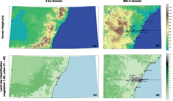
Figure 1. WRF domain configuration for the parent domain at 4 km resolution ((a) and (c)) and nested domain at 800 m resolution ((b) and (d)). For terrain height (m) ((a) and (b)), and dominant land use classification ((c) and (d)) where the urban types correspond to values 31 (LCZ1) to 40 (LCZ 10). AWS site locations (annotated black dots) and the East–West transect (dashed black line) are identified for the nested domain ((b) and (d)).
Download figure:
Standard image High-resolution imageThere are 45 hybrid eta vertical levels from the surface to 50 hPa for the atmospheric model. A 10 s timestep for the outermost parent domain is used and a reduced timestep at a ratio of 3:1 for the nested domains. The lateral boundary conditions for the parent domain and sea surface temperatures are sourced from the 6 hourly 70-level Bureau of Meteorology Atmospheric high-resolution Regional Reanalysis for Australia (BARRA) available at 12 km resolution (Su et al 2019). During early 2017 southeast Australia experienced persistent hot temperatures with frequent heatwave events. A five-member initial condition ensemble is run for the period 1 January 2017 until 28 February 2017 with initialization of the individual ensemble members starting at 6 h intervals.
2.2. Urban typology and parameter estimation
For the urban grid points we use the World Urban Database Access Portal Tool (WUDAPT) (Brousse et al 2016) to create an urban classification map for Sydney following the urban types described by the local climate zones (LCZs) of Stewart and Oke (2012). Using the tools developed by Brousse et al (2016) the ten urban types (table 1) are integrated into the landcover classification of WRF (figure 1). Urban areas not covered by our Sydney LCZ map that are within the nested domain were modeled as a compact low-rise urban form.
Table 1. Urban parameters used for the Sydney LCZs in WRF.
| LCZ | Type | Building height (m) median (std dev) | Albedo (−) | Vegetation fraction (%) | Anthropogenic heat (W m−2) |
|---|---|---|---|---|---|
| 1 | Compact high-rise | 80 (67.58) | 0.107 | 3.7 | 54.0 |
| 2 | Compact mid-rise | 16 (20.96) | 0.134 | 17.8 | 20.1 |
| 3 | Compact low-rise | 8.5 (0.59) | 0.146 | 25.9 | 12.4 |
| 4 | Open high-rise | 35 (44.46) | 0.134 | 8.9 | 54.0 |
| 5 | Open mid-rise | 16 (20.96) | 0.134 | 8.9 | 20.1 |
| 6 | Open low-rise | 9 (0.54) | 0.148 | 32.7 | 10.5 |
| 7 | Lightweight low-rise | 4 (1.32) | 0.160 | 60.4 | 5.4 |
| 8 | Large low-rise | 9 (2.18) | 0.158 | 22.4 | 11.7 |
| 9 | Sparsely built | 10 (0.60) | 0.156 | 73.1 | 3.6 |
| 10 | Heavy industry | 11 (2.47) | 0.161 | 23.4 | 63.9 |
Updating the urban types within WRF requires appropriate estimation of parameters to describe key attributes of each type (table 1). Here we use the Urban Vegetation Cover and Environmental Planning Instrument—Height of Buildings datasets maintained by the New South Wales Government Department of Planning, Industry and Environment (DPIE 2008, 2019) to estimate the vegetated fraction and building height respectively for each urban type. We use the MODIS Bidirectional Reflectance Distribution Function Albedo data (Schaaf and Wang 2015) to estimate building albedo and the anthropogenic heat emission global database by Dong et al (2017) to estimate the anthropogenic heat flux. To estimate the parameters, we extract the points corresponding to each LCZ type from the respective database and calculate the median and standard deviation. The final estimates are presented in table 1 and are within the ranges defined by Stewart and Oke (2012).
2.3. Observational data and model evaluation
Due to the high resolution of the WRF simulations, evaluation of the model skill against gridded climate data is challenging. Therefore we use observations from 11 automatic weather stations (AWS) maintained by the Australia Bureau of Meteorology that have data for the simulation period within the model domain (figure 1). These data are available at a 1 min interval and are aggregated to 10 min averages. We extract the model outputs co-located with the geographic location of the AWS sites and compare the 10 min time series. To quantify the simulation skill we use the metrics of the International Land Model Benchmarking system (Collier et al 2018) which includes metrics of the relative bias, the root mean square error and the phase skill score (see supplementary material (available online at stacks.iop.org/ERL/16/064066/mmedia)). An example of the time series comparison for Sydney Airport is provided in supplementary figure S1 with the skill scores for various variables across all AWS sites included in supplementary tables S1 and S2. Overall, the model skill is high, although precipitation events were limited over January-February 2017 there remain limitations in the timing and magnitude of precipitation events. Additional assessment of the differences between urban and non-urban outputs is provided in supplementary figures S2 and S3.
2.4. Heatwave identification
To identify the heatwave days during January/February 2017 we use observational station data from Sydney Airport (66037), as well as Observatory Hill (66062) and Richmond (67105) stations that are part of the Australian Climate Observations Reference Network—Surface Air Temperature (ACORN-SAT) maintained by the Australia Bureau of Meteorology. Although many definitions exist for heatwave identification, we use a modified version of the excess heat factor originally defined by Nairn and Fawcett (2013) that implicitly incorporates a seasonal cycle to characterize heatwaves according to the climatological conditions for a particular time of the year (Perkins and Alexander 2013). Heatwave days are identified by calculating the anomaly in the daily mean temperature (determined from the average of the daily maximum and minimum temperature) above the calendar day 90th percentile (equation (1)). By using the daily average temperature, we can account for the impact of warm nights as well as warm days during heatwave events. When the daily average temperature anomaly is positive for at least three consecutive days, these are classified as heatwave days.
Here T90 is calculated using a 15 day window centered on the corresponding calendar day with a temperature T1 for the standard climatological reference period of 1961–1990. This definition has been used previously to identify Australian heatwave events in Hirsch et al (2019) and Hirsch and King (2020). Applying this definition to the weather station data, we identify five heatwave events that occurred in quick succession over Sydney during January-February 2017. Using a slightly different definition based on maximum daily temperatures yielded comparable heatwave day identification.
3. Results
3.1. Temporal evolution of local breezes during a heatwave season
We assess the temporal evolution of the urban gradient along an East–West transect, from coast to inland, of the temperature, moisture content, and horizontal wind speed components (figure 2). Across the simulation period the temperature gradient across the city varies with a mean value of 0.83 °C and a maximum value of 15.79 °C. The largest temperature gradients (figure 2(a)) often occur during the heatwave events when there is a westerly flow over the Blue Mountains located west of the city (figure 2(c); positive u-wind component). More specifically, at instances where there is an abrupt change to a westerly flow at the urban/rural interface, corresponding to the dates 11 January 2017, 17 January 2017, 30 January 2017 and 10 February 2017, an easterly flow at the coast is present. This contributes to the establishment of large temperature gradients due to the relatively cooler conditions present at the coast. This is also observed in available data from the weather stations (supplementary figure S4). A closer examination of the time series for the first heatwave event (supplementary figure S5) shows that there are instances where the v-wind direction is different between coastal grid cells and those further inland. More specifically on the 11 and 13 January the v-wind is Southerly at the coast and Northerly further inland, which would also contribute to the development of the large temperature gradients observed on those days.

Figure 2. Time series across the lowest atmospheric level over the urban area along an East–West transect at latitude 33.85° S for: (a) temperature (T; °C), (b) water vapor (Q; kg kg−1), (c) u-wind velocity (U; m s−1; positive is from the west), and (d) v-wind velocity (V; m s−1; positive is from the south). The vertical shaded areas indicate the five heatwave periods as determined from long-term daily temperature observations at Sydney Airport, Observatory Hill, and Richmond. There is one line for each urban grid cell with values closer to red corresponding to the grid cells further inland and lines closer to blue corresponding to grid cells closer to the coast. Shorter time series coinciding with each heatwave event are available in supplementary figures S5–S9.
Download figure:
Standard image High-resolution imageA recurrent feature during the simulation is the sea breeze (figure 2(c); negative u-wind component) which contributes to ventilating the city and reducing the temperature gradient (figure 2(a)). The second heatwave is the only event where a strong westerly flow does not occur at the onset but is present during the event. Instead, the south-easterly air flow contributes to delaying the transport of the warmer inland flow across the whole city to the second heatwave day. The timing of this event is sensitive to the station data used, with a one day difference in the onset timing between the inland Richmond and coastal Observatory Hill site. This is likely associated with the easterly flow that persists over the 14 and 15 January preceding the second heatwave event. This is indicative of how influential sea breezes can change the onset timing of a heatwave across a large coastal city. All heatwave terminations are coincident with a strong southerly flow (figure 2(d); positive v-wind component) that cool temperatures across the city.
Examining the radiative changes across the transect (supplementary figure S11) indicates that the downward short- and longwave radiation is generally consistent across the city. Furthermore, over the days preceding each heatwave event, the smooth time series of the downwards shortwave radiation are indicative of the clear sky conditions that develop at heatwave onset. Given the temperature increases over the same days that clear sky conditions occur prior to each heatwave, we are confident that the timing of the heatwave events are consistent with the observed days.
3.2. Conditions at heatwave onset
Most of the heatwaves commence with heat transport into the region from the west to north-west of Sydney with cooler conditions over the adjacent ocean surface (figure 3). This confirms how large gradients can establish over the city by the contrasting temperatures between the continental interior and the adjacent ocean. For the first heatwave, surface wind speeds over the adjacent ocean are weak compared to subsequent heatwave events where a strong southward flow persists. The contrasting wind directions and temperature gradient across the city (figure 2(c)) are attributed to how the large-scale flow influences heat dispersion. For example, the third heatwave commences with the convergence of strong surface wind (figure 3(d)) which results in strong updrafts close to the coastline (figure 3(m)). For the second heatwave, the southward flow extends over the city to inhibit the transport of dry air from the west into the city, although the urban footprint of Sydney is still evident with a temperature of 28 °C–30 °C compared to 24 °C–26 °C over the surrounding vegetated areas (figure 3(b)). The moisture contrast between the ocean and the land is anticipated however for the 3rd and 4th heatwaves the moisture content increases along the coastline coincident with the convergence of the continental westerly flow and oceanic southward flow. Examining the impact of the urban environment for heatwave onset (supplementary figure S12) shows that the city contributes to hotter onset for the first three events, drier surface conditions for all events, and can induce intense thermal updrafts.
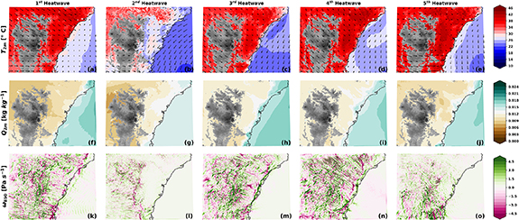
Figure 3. Contour maps of the conditions at the onset of the five Sydney heatwaves during January–February 2017. For (a)–(e) 2 m air temperature (T2m; °C; shaded) and 10 m wind (vectors), (f)–(j) 2 m moisture content (Q2m; kg kg−1; shaded), and (k)–(o) the vertical motion at 850 hPa (ω850; Pa s−1; positive upwards). For the first (a), (f), and (k), second (b), (g), and (l), third (c), (h), and (m), fourth (d), (i), and (n), and fifth (e), (j), and (o) heatwave. Panels (a)–(j) include the model topography above 650 m shaded in grey.
Download figure:
Standard image High-resolution image3.3. UHI amplification during heatwaves
To evaluate the UHI contribution we compare the WRF output over January–February 2017 between simulations where the urban parameterization is activated against those where all urban areas are represented as grasslands (hereafter referred to as non-urban simulations). The UHI is a persistent feature during the simulations with a mean value of 1 °C over the city that extends west over the Blue Mountains (∼0.5 °C) up to a depth of 1 km into the atmosphere from the surface (figure 4(a)). This is accompanied by a drier atmospheric profile (∼0.003 kg kg−1) with a comparable extent to the temperature amplification (figure 4(b)). The drier atmosphere is attributed to a decrease in moisture supply from the land surface as the contribution from evapotranspiration is significantly reduced when the urban parameterization is activated due to the smaller vegetation fractions.

Figure 4. Ensemble mean difference over January–February 2017 between urban and non-urban realizations along an East–West transect through the nested domain (at latitude 33.85° S) comparing the vertical profile of (a) temperature (T; °C), and (b) water vapor (Q; kg kg−1). The black shaded region depicts the topographic profile and the colored line along the x-axis denotes the surface type (green = vegetated, grey = urban, and blue = ocean).
Download figure:
Standard image High-resolution imageThere is considerable variability in the strength and extent of the UHI as determined by the prevailing airflow across the region (not shown). In particular, there is further extension over the Blue Mountains of the UHI when the airflow is easterly, and when the airflow is westerly, the UHI temporarily extends over the adjacent ocean. Over January–February 2017, the UHI has a diurnal cycle with an average daytime UHI of 0.65 °C and an average nighttime UHI of 1.58 °C across the city.
Due to the reduced efficacy of sea breezes to ventilate the whole city during the heatwave events (figure 2) the cumulative heat attributed to the urban environment over the five heatwave events, calculated as the sum of the mean daily temperature difference divided by the number of heatwave days, increases to more than 10 °C over the city and 3 °C further west of the city over the Blue Mountains (supplementary figure S13). Again, the UHI has a larger impact at night, with an average night-time cumulative heat of 8.01 °C over the city during the five heatwave events, compared to a daytime cumulative heat of 3.89 °C.
3.4. Contrast across urban types
To examine whether the UHI effect varies between the urban types we compare the diurnal variations in temperature, humidity and wind speed (figure 5). By considering the difference of the urban from the non-urban simulations, we can account for the effect of distance from the coast as some urban types are predominantly coastal (e.g. compact high-rise) compared to others. For air temperature (figure 5(a)), dew-point temperature (figure 5(b)) and relative humidity (figure 5(c)), the heavy industry, large low-rise and sparsely built urban classes show a greater diurnal variability compared to the compact and open urban classes. The compact urban classes and open high-rise are consistently warmer than non-urban areas at all times of the diurnal cycle, whereas the remaining urban classes are predominantly warmer than non-urban types at night. (figure 5(a)). For all urban classes the relative humidity is lower at all times, consistent with figure 4(b), however the moisture deficit is larger at night. The wind speed (figure 5(d)) is increased over most urban areas at night and decreased during the day between 0900 and 1600 for all urban classes. The diurnal variation can be attributed to how the urban environment establishes the strength of the temperature gradient across the city. More specifically, as more heat is retained by the thermal mass of the urban environment, large thermal contrasts between the city and adjacent ocean contribute to the strength of both land and sea breezes. Therefore, as a result of the larger thermal gradient at night between urban and non-urban simulations, irrespective of the urban class, higher wind speeds occur.

Figure 5. Contrast between urban types over the diurnal period for (a) 2 m air temperature (T2m; °C), (b) 2 m dew point temperature (Tdp; °C), (c) 2 m relative humidity (RH; %), and (d) 10 m wind speed (WSPD; km h−1). Each vertical line corresponds to the inter-quartile range for the change (urban minus non-urban) in the quantity for urban types at a given hour of the day. Only grid cells where the fraction of the urban type exceeds 50% of the grid cell are included.
Download figure:
Standard image High-resolution image
4. Discussion
By performing convection permitting simulations at 800 m resolution over Sydney we are able to resolve the temperature and moisture gradients that establish across the city during heatwave events. These arise as a consequence of the convergence of hot and dry continental flow over the Blue Mountains west of Sydney and southward cooler flows over the adjacent ocean. In particular, the Foehn-like conditions that occur at the onset of, and during, the heatwaves are an important mechanism for heat accumulation. Independent analysis by Abatzoglou et al (2020) identifies Foehn events from the ERA-5 reanalysis based upon three criteria defined by the cross-barrier wind speed, vertical motion and the atmospheric lapse rate. Using the Foehn database of Abatzoglou et al (2020), 14 Foehn events occurred over the Greater Sydney region during January–February 2017. When Foehn events occur, mean temperature across the city can increase by between 10.17 °C (20 January) and 21.79 °C (11 February) over a 24 h period. The sea breeze is a recurrent feature and is detected every day with temperature gradients across the city decreasing to within 1 °C at its peak. When synoptic systems pass across the domain, particularly at the termination of the heatwave events, temperatures across the city can decrease rapidly. For example, the termination of the second heatwave (19 January) coincided with a Southerly Buster event with mean temperature across the city decreasing by 11.43 °C over a 24 h period. These conditions are clearly resolved across the domain with figure 2 suggesting that both Foehn and sea breeze phenomena impact conditions across the city with some variation in timing and magnitude.
Further to the Foehn conditions transporting heat into the city, the UHI enhances the heat accumulating over the city region. In particular, the built environment contributes to a warmer and drier boundary layer, a consequence of how urban areas modify radiative exchange, heat storage and the hydrological cycle. Furthermore, the UHI extends beyond the city limits arising from the local flows that advect heat around the region. During the heatwave events, the UHI contributes to a cumulative heat of 10 °C that has limited capacity to dissipate given the convergence forming at the coast due to relatively stronger offshore flows. Therefore the warming is not contained at the surface layer, with subsequent convection dispersing the heat within the lower atmosphere.
Observations for Sydney demonstrate that the thermal contrast across the city increases during heatwave events that dissipate with strong sea breezes and southerly flows (supplementary figure S4). However the convection-permitting WRF simulations provide the four-dimensional wind, temperature and moisture profile across the city to understand how conditions evolve and propagate across the whole city rather than at a few discrete locations. In particular, the contrast across the city is more than a function of distance from the coastline, with temperature gradients often 2 °C–4 °C lower in the non-urban simulations particularly for inland parts of the city (supplementary figure S14). Furthermore, differences between the urban and non-urban outputs for temperature, moisture content and wind are larger further inland than at the coast. Therefore, the representation of the urban areas is critical for simulating both the gradient across the city and the UHI.
The experimental setup consisted of two domains at 4 km and 800 m enabling an assessment of skill gains from the resolution. The evaluation of simulation skill to weather station data (supplementary tables S1 and S2) indicate that the 800 m resolution outputs have greater skill in simulating the temporal variability of mean sea level pressure, 2 m air temperature and 10 m wind speed. Examining differences in the spatial variability against observational data is challenging as gridded observations for this region are derived from the weather station data and therefore these products are sensitive to the underpinning spatial distribution of the sites. Remote sensing products for temperature are available, however ideally assessment of hydrological variables is necessary to determine the robustness of changes in the skill of capturing the spatial variability. Instead, kernel density functions were used as a nonparametric estimate of the underpinning probability distribution comparing 4 km and 800 m resolution outputs between day and night (supplementary figure S15) and heatwave and non-heatwave days (supplementary figure S16). This reveals that there are statistically different distributions for 2 m air temperature and moisture content and 10 m wind speed as a consequence of differences in the resolution. Regarding recommendations on resolution, the 4 km may be sufficient to resolve UHI at the city scale, while 800 m is more appropriate for resolving the contrast between urban types within the city.
Our results are consistent with previous research that has demonstrated UHI amplification during heatwave events for cities in China (Jiang et al 2019) and the United States (Zhao et al 2018). In particular, Jiang et al (2019) found that the amplification was associated with changes in how effective sea breezes ventilated the city, as shown by our results for Sydney. Mughal et al (2019) use the LCZs to describe the urban environment of Singapore and identify diurnal variation in UHI intensity across the different urban classes. For Singapore, compact high-rise had a larger UHI intensity than other LCZ types (Mughal et al 2019) which contrasts with our results showing greater intensity from heavy industry. This may be associated with differences in the composition and distribution of the different LCZ urban classes between Sydney and Singapore. Therefore, acknowledging that differences in city composition will have an impact on the UHI, our results for Sydney are broadly comparable to what has been demonstrated previously.
Our high-resolution experimental setup facilitated the evaluation of how urban heat varies across urban types irrespective of proximity to the coastline. This offers valuable insights for urban planning of Sydney in response to future development associated with population growth. Our results suggest that the diurnal cycle of the UHI is smaller for more compact urban forms with larger diurnal variation for heavy industry and sparsely built urban forms. For heavy industry, this is associated with changes in anthropogenic heat emissions and for sparsely built areas, the larger diurnal variation corresponds to variations in evapotranspiration which can have large contrasts between day and night. Future research aimed at examining different scenarios for areas zoned for future development may prove useful for urban planners to determine tradeoffs between different development pathways.
5. Conclusion
Computational advances have been fundamental for the execution and interrogation of convection-permitting simulations at 800 m resolution over Sydney, Australia. At this high-resolution, the flows arising from both the complex topography and the comprehensive representation of the urban form provide a powerful tool for examining how UHIs grow during heatwave events. We have demonstrated that resolving the complexity of urban environments is essential for quantifying city gradients and how local flows influence their variability. Further research into how changes in the urban environment along with climate change are required to understand how local and global forcings co-evolve. This is a necessary step for providing high-resolution projections aimed at building city resilience to the challenges arising from both urban expansion and climate change.
Acknowledgments
The computational modeling was supported by the National Computational Infrastructure (NCI) at the Australian National University in Canberra, Australia. This project is supported through funding from the Australian Research Council (ARC) Centre of Excellence for Climate Extremes (CE170100023).
Data availability statement
The data that support the findings of this study are available upon reasonable request from the authors.
Code availability
The WRF model code is open access and available from https://github.com/wrf-model/WRF. The analysis code is available at https://github.com/annettehirsch/hirsch_wrf-urban.git.
Author contributions
A L H and J P E conceived the study. A L H implemented the urban classification in WRF, performed the model simulations and data analysis. J P E contributed to designing the experiments. C T prepared the tools for creating the WRF boundary conditions from BARRA and the preliminary design of the WRF configuration. J L, B C, and M A H developed the urban classification map of Sydney. M L, M A H and A L H estimated the parameters for the Sydney urban classification. W E evaluated differences between the domains for resolution dependence. All authors contributed to the manuscript writing and editing.