

Abstract
Drought is one of the most extreme climatic events in South Asia (SA) and has affected 1.44 billion people in last 68 years. The agriculture in many areas of this region is highly dependent on rainfall, which increases the vulnerability to drought. To mitigate the impact of drought on agriculture and food security, this study aims to develop a state-of-the-art system for monitoring agricultural drought over SA at a high spatial resolution (0.25∘) in near real-time. This study currently focuses on the rain-fed area, and the impact of irrigation is not incorporated. This open and interactive tool can assist in monitoring the near-present soil moisture conditions, as well as assessing the historical drought conditions for better management. The South Asia Drought Monitor (SADM) runs the mesoscale hydrologic model to simulate the soil moisture using observation-based meteorological forcing (at near real-time), morphological variables, and land cover data. The soil moisture index (SMI) has been calculated by estimating the percentile of the simulated soil moisture. The drought monitor displays the SMI in five classes based on severity: abnormally dry, moderate drought, severe drought, extreme drought and exceptional drought. The main functions of this open interactive system include the provisioning of up-to-date and historical drought maps, displaying long-term drought conditions and downloading soil moisture data. Comparison of the SMI with the standardized precipitation evapotranspiration index (SPEI) shows that the SMI and SPEI depict similar temporal distribution patterns. However, the SPEI (for 4, 6, 9 and 12 months) differs in the representation of the dry conditions in 1992, 2009, and 2015 and the wet condition in 1983, 1988, and 1990. We evaluated the implications of using different precipitation forcings in a hydrological simulation. A comparison of major drought characteristics such as areal extent, duration, and intensity, using different precipitation datasets show that uncertainty in precipitation forcings can significantly influence model output and drought characteristics. For example, the areal extent of one of the most severe droughts from 1986 to 1988 differs by 9% between ERA5 and CHIRPSv2.
Export citation and abstract BibTeX RIS

Original content from this work may be used under the terms of the Creative Commons Attribution 4.0 license. Any further distribution of this work must maintain attribution to the author(s) and the title of the work, journal citation and DOI.
1. Background
Drought is a natural climate phenomenon that has devastating impacts on food security, water resources, ecosystems, health, energy, and the economy (Wilhite et al 2000, FAO 2018). Since the 1950s, the frequency of heatwaves and intense droughts has increased in many regions of Africa, America, Asia, Australia, and Europe (IPCC 2012). South Asia (SA) is one of the most populated regions on Earth; approximately 25.87% of the world population lives in this region (World Population Review 2020). Out of the South Asian countries, Afghanistan, India, Pakistan, and Sri Lanka each experienced one drought every three years over the past five decades, and Bangladesh and Nepal also suffered from frequent droughts (Miyan 2015, Aadhar and Mishra 2017). In Afghanistan, a severe drought in 2011 affected 2.6 million people across 14 provinces (Qamer and Matin 2019). In India, droughts in 1987, 2002, 2003, and 2010 affected more than 40% of the country (Kumar et al 2013). Bangladesh experienced extreme droughts in 1973, 1978, 1979, 1981, 1982, 1989, 1992, 1994, 1995, 2006, and 2009 (Hossain 1990, Habiba et al 2012, Mia 2014). Overall, from 1950 to 2018, 42 droughts have occurred in SA, affecting 1.44 billion people, and causing damage amount to approximately 5.88 billion U.S. dollars (EM-DAT 2020). Thus, it can be expected that droughts will continue to affect the South Asian region.
The agriculture of SA is largely dependent on rainfall, although 46% of the cultivated area is under irrigation (FAO 2012). Change in rainfall patterns and/or temperature can negatively affect the agricultural production in the region. For example, in Bangladesh, droughts in 1979 and 1982 led to a decline in rice production by approximately 2 million tons and 53 thousand tons, respectively (Selvaraju et al 2006). The 2008–2009 winter drought in Nepal was one of the worst on record, when the country received less than 50% of its average precipitation. This led to a decrease in wheat and barley production by 14.5% and 17.3%, respectively (Joint Assessment Report 2009). Approximately 57% of the land area in SA is used for agriculture, and nearly 60% of the population works in the field of agriculture (AFA 2019). This high dependency on rain-fed agriculture makes SA vulnerable to droughts, their intensity, duration, and areal extent.
Drought monitoring and forecasting are crucial for mitigating the detrimental impacts of droughts. The policymakers and water managers of this region face difficulties in dealing with droughts owing to a lack of reliable data as well as insufficient technical and institutional capacities (Thenkabail et al 2004, Global Water Partnership 2014, Aadhar and Mishra, 2017). In most of the countries in SA, drought forecasting is not as high a priority as mitigating flood damage; however, India has advanced drought monitoring and forecasting technology (Mirza 2010). The India meteorological department (IMD) began drought monitoring for India (www.imdpune.gov.in/hydrology/Drought_Monitoring.html) in 1967. This tool monitors meteorological drought based on the aridity anomaly index and the standardized precipitation index (SPI). An Experimental Drought Monitor (https://sites.google.com/a/iitgn.ac.in/india_drought_monitor/home) was developed in 2014 to provide near real-time drought information in India at a spatial resolution of 0.25∘ by estimating the SPI, standardized runoff index (SRI), and standardized soil moisture index (SMI) (Shah and Mishra 2015). This portal provides drought information from 2014–2017 and later started providing drought information for the whole of SA as the 'High Resolution South Asia Drought Monitor'. Since 2004–2005, the Pakistan meteorological department (PMD) have been providing fortnightly and monthly drought condition analysis (www.ndmc.pmd.gov.pk/NDMC-Latest-Drought-Advisory.php) using rain gauge data and a satellite-based vegetation index.
On the regional scale, the satellite-based drought monitoring and warning system (http://wtlab.iis.u-tokyo.ac.jp/DMEWS/) tracks meteorological drought conditions over cropland in Asian countries by estimating the Keeth–Byram Drought Index (KBDI) using satellite-based rainfall, temperature, and vegetation phenology (Takeuchi et al 2015). The South Asia drought monitoring system (SADMS) (http://dms.iwmi.org/maps_and_data.php) is the first drought monitor for SA. Established in 2014, the SADMS provides a weekly map of drought conditions at a spatial resolution of 0.5 km by 0.5 km in near real-time. This system monitors drought by calculating the integrated drought severity index based on satellite-based observations of vegetation conditions, climate data, and other biophysical information (Amarnath et al 2019, IWMI n.d.). Aadhar and Mishra (2017) identified the need for monitoring drought at a high resolution in near real-time to improve the decision-making process. Subsequently, the high resolution South Asia drought monitor (SADM) (https://sites.google.com/a/iitgn.ac.in/high_resolution_south_asia_drought_monitor/) was developed. This system monitors drought by estimating the SPI, SRI, and SSI using satellite-based precipitation data at a 0.25∘ (SPI at 0.05∘ and 0.25∘) spatial resolution. Recently, ICIMOD has developed the Regional Drought Monitoring and Outlook (http://tethys.icimod.org/apps/regionaldrought/) using five variables (soil moisture, precipitation, air temperature, evapotranspiration and SPI) from the SALDAS dataset, where the SALDAS data use satellite-derived precipitation and land cover information (SERVIR n.d.).
The current approaches to drought monitoring in SA are based on different drought indices, satellite imagery, and hydrological models, in which data are obtained from in situ observations and various satellite-based sources. The existing platforms play an important role in information dissemination and drought management. However, underlying scientific and technical challenges, such as inconsistent data, uncertainty in hydrological models, and sensor changes, might affect the monitoring and forecasting of droughts. For example, some studies recommend remote sensing as a potential technology for drought monitoring in SA because the spectral resolution can provide information about vegetation condition (Thenkabail et al 2004, Vadrevu et al 2019). Notably, there are challenges in using satellite products, e.g. relatively short record lengths, temporal inconsistency due to changes in sensors, and indirect ways of retrieving physical variables (Sheffield et al 2014). Conversely, hydrological models are suitable tools that provide a realistic depiction of soil moisture by simulating land-atmospheric fluxes and hydrologic processes. However, uncertainty in these model outputs can be created by the model parameters, model structure, and input data (Decharme and Douville 2006, Samaniego et al 2013, Nair and Indu 2018). In SA, especially in the Hindu Kush Himalayan Region (figure 1), meteorological data are known to be the primary source of uncertainty in the model simulated output (Ghatak et al 2018). Using station-based data in this region is also challenging because of the sparse distribution of rain gauges, incomplete historical records, and a lack of up-to-date freely accessible sources.
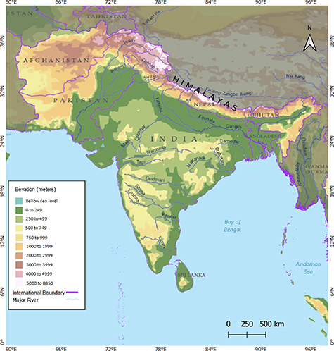
Figure 1. Physiography, rivers and countries of South Asia (source: Esri, Garmin, CIA World Factbook 2015, Esri 2016, NOAA, Maps.com 2016).
Download figure:
Standard image High-resolution imageThis study presents the SADM, that has been developed for monitoring agricultural drought at a high-resolution (0.25∘) and in near real-time (5 days latency). Currently, the system provides information for rain-fed agriculture, and data on irrigation is not included. Additionally, this tool can be used for historical drought assessment; understanding the past drought events and resulting impacts can assist the decision-makers in implementing more informed drought risk management strategies. The study also compares a model-derived soil moisture drought index to a meteorological drought index for agricultural drought estimation. Furthermore, the uncertainty created by different precipitation forcings in simulated soil moisture is analyzed. This drought monitoring system intends to provide near real-time drought information to the water managers, policy-makers, politicians, stakeholders from relevant public and private sectors, and the general public.
2. Overview of the approach
The SADM has been developed for seven countries in SA (Afghanistan, Bangladesh, Bhutan, India, Nepal, Pakistan and Sri Lanka), covering the four major river basins of SA, namely the Indus (1120 000 km2), Ganges (1087 300 km2), Brahmaputra (543 400 km2), and Meghna (82 000 km2) (FAO 2012) (figure 1). The SADM is inspired by the German Drought Monitor (www.ufz.de/index.php?en=37937) (Zink et al 2016). The SADM estimates daily and monthly agricultural drought conditions using the mesoscale hydrologic model (mHM) (www.ufz.de/mhm) (Samaniego et al 2010, Kumar et al 2013). The overall framework of the system comprises three basic steps (figure 2). First, the mHM is implemented to reconstruct daily and monthly soil moisture using historical meteorological forcings (at near real-time), morphological variables, and land cover data. Second, the SMI is estimated with a non-parametric kernel-based cumulative distribution function (Samaniego et al 2013) based on the mHM's historic soil moisture reconstruction. The generated SMI maps are separated into five classes based on severity: abnormally dry, moderate drought, severe drought, extreme drought and exceptional drought. The drought classification has been adapted from the US Drought Monitor (Svoboda et al 2002). Third, the SADM is developed, which is an interactive web-platform (http://ufzchs.pythonanywhere.com/) for the dissemination of the simulated near real-time drought conditions. To achieve maximum dissemination, the daily and monthly SMI fields are uploaded every day and published on the SADM portal.

Figure 2. Framework of the South Asia Drought Monitor. Reproduced from Saha et al (2020). CC BY 4.0.
Download figure:
Standard image High-resolution image2.1. Reconstruction of soil moisture using mHM
The mHM is used to reconstruct the daily and monthly soil moisture. The mHM is a spatially distributed, grid-based hydrologic model that considers grid cells as a primary modeling unit (Samaniego et al 2010, Kumar et al 2013) and simulates the following processes: canopy interception, snow accumulation and melting, soil moisture dynamics, infiltration and surface runoff, evapotranspiration, subsurface storage and discharge generation, deep percolation and baseflow, and discharge attenuation and flood routing. The uniqueness of the model is the application of the multiscale parameter regionalization technique, that accounts for the sub-grid variability of physiographic characteristics (Samaniego et al 2010, Kumar et al 2013). The mHM has been successfully implemented for all major river basins in Germany (Zink et al 2017), for 400 European river basins (Rakovec et al 2016) and across the continental United States (Rakovec et al 2019). Through this research, the mHM is used for the first time to monitor drought in SA.
In order to evaluate the uncertainties in soil moisture simulation associated with precipitation forcing, we use three gridded precipitation products at a 0.25∘ resolution, namely, Princeton Global Forcings v3.0 (PGFv3, Sheffield et al 2006), Climate Hazards Group InfraRed Precipitation with Stations v2.0 (CHIRPSv2, Funk et al 2015), and a fifth-generation product ECMWF Atmospheric Reanalysis (ERA5, Copernicus Climate Change Service 2017) from 1982 to 2016. For all reconstructions, we use PGFv3 temperature data from 1982 to 2016 at a 0.25∘ resolution. Other inputs such as terrain elevation, soil, geology, land cover, and leaf area index (LAI) data also remained unchanged.
The near real-time soil moisture simulations of the SADM are based on the ERA5 Reanalysis dataset (precipitation and temperature) at a 0.25∘ spatial resolution. ERA5 datasets are available from 1979 to present with a 5 day latency. Based on the availability of a higher resolution dataset with less latency, this tool will be upgraded. The ERA5 dataset combines significant amounts of historical observations into global estimates using advanced modeling and data assimilation methods (Copernicus Climate Change Service 2017). Other required variables (terrain elevation, soil, geology, land cover, and LAI) are collected from various sources (table 1) to determine the physical characteristics of the basin. The mHM model performance has been successfully evaluated against a time series of monthly terrestrial water storage anomalies from the GRACE satellite (Landerer and Swenson 2012) and gridded FLUXNET evapotranspiration product (Jung et al 2011, see figure A1).
Table 1. Data used in for South Asia drought monitor.
| Data type | Dataset name | Processed resolution | Author |
|---|---|---|---|
| DEM (+ derivatives) | Global multi-resolution terrain elevation data (GMTED2010) | 1/512∘ | U.S. Geological Survey (USGS) |
| Soil | SoilGrids | 1/512∘ | ISRIC—World Soil Information (2017) |
| Geology | Global lithological map (GLiM) | 1/512∘ | Hartmann and Moosdorf (2012) |
| Land cover | Global land cover (GlobCover) | 1/512∘ | European Space Agency (ESA), Universit Catholique de Louvain (2009) |
| LAI | Global inventory modeling and mapping studies (GIMMS) | 1/512∘ | Tucker et al (2004) |
| Precipitation and temperature | ERA5 | 0.25∘ | Copernicus Climate Change Service (2017) |
For the SADM, agricultural drought is estimated in terms of low soil moisture values. The mHM estimates the soil moisture based on soil water availability at six different depths (5, 15, 30, 60, 100, and 200 cm), which is considered to be the root zone (Kumar et al 2013, Zink et al 2016). Following Samaniego et al (2018), we use the mean volumetric soil moisture averaged over these six soil layers. To reconstruct the soil moisture, we ran the simulation from 1980 to near-present. The system is currently running, and it estimates the daily and monthly soil moisture in near real-time with a 5 day latency.
2.2. Calculation of soil moisture index (SMI)
The simulated soil moisture is then used to estimate SMI, which represents the soil moisture deficit compared to the seasonal climatology of that particular area. SMI is calculated by estimating the quantile of soil moisture for a particular month and grid cell with respect to its kernel-based cumulative distribution function generated from the historical simulations. The methodology for estimating the SMI from soil moisture values has been adapted from Samaniego et al (2013). The SMI values are estimated for the entire record from 1980 to near real-time. The values are represented in a range of 0–1, where a value close to zero indicates areas with higher water deficit, and a value close to one represents wet soil moisture conditions. We estimate the SMI values using the soil moisture output of three precipitation products: CHIRPSv2, ERA5 and PGFv3; the respective SMIs are denoted as CHIRPSv2-SMI, ERA5-SMI, and PGFv3-SMI, respectively. The SMI values are categorized into five classes, namely, abnormally dry, moderate drought, severe drought, extreme drought, and exceptional drought (table 2) using the thresholds of the SMI (adapted from Svoboda et al 2002).
Table 2. Classification of droughts for the South Asia drought monitor based on the soil moisture index (SMI) (adapted from Saha et al 2020).
| SMI class | Drought condition | Chance of occurrence | Possible impacts |
|---|---|---|---|
0.2  SMI SMI  0.3 0.3 | Abnormally dry | 21%–30% | Slowing down of crop and pasture growth |
0.1  SMI SMI  0.2 0.2 | Moderate drought | 11%–20% | Some damage to crops and pastures |
0.05  SMI SMI  0.1 0.1 | Severe drought | 6%–10% | Crop or pasture losses likely |
0.02  SMI SMI  0.05 0.05 | Extreme drought | 3%–5% | Major crop/pasture losses |
SMI  0.02 0.02 | Exceptional drought | 2% or less | Exceptional and widespread crop/pasture losses |
2.3. Data dissemination through SADM
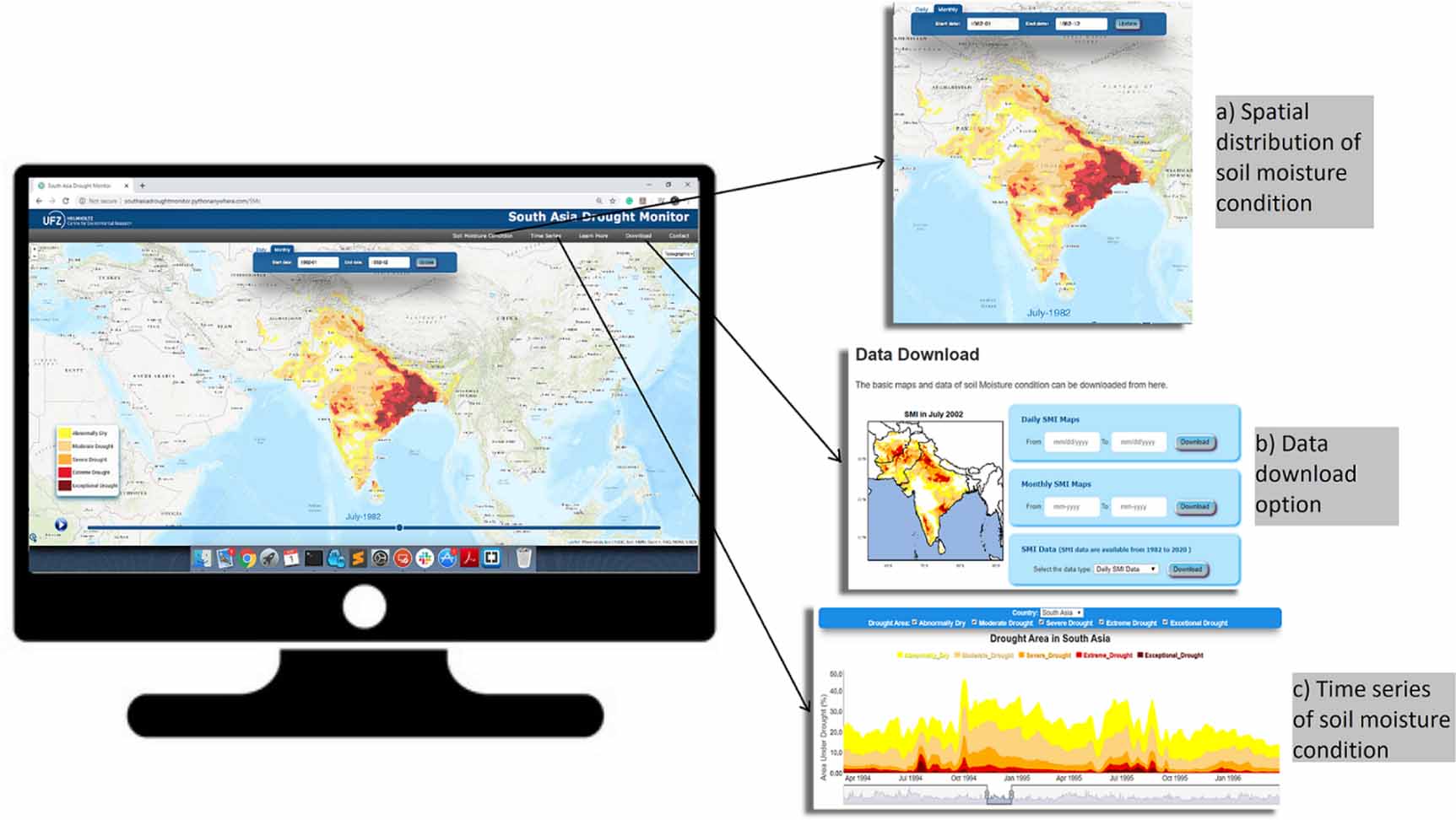
One of the important parts of developing a monitoring system is to ensure efficient dissemination of drought information. For this reason, an open and interactive web-based tool, SADM (http://ufzchs.pythonanywhere.com/), has been developed, where users can access the map and time series of daily and monthly drought conditions from 1980 to five days before real-time. Users can also download the drought maps, times series plot of the areal extent, and SMI data (daily and monthly) for the aforementioned period. Figure 3 shows the snapshots of different interfaces of SADM.

Figure 3. Key features of the South Asia drought monitor: an interactive interface to display and animate drought maps from 1980 to 5 days before real-time (a), a download facility to obtain drought maps and SMI data (b), and interactive time series plots of drought condition from 1980 to the current year (c).
Download figure:
Standard image High-resolution image'Leaflet' library (https://leafletjs.com/) of JavaScript is used to display interactive drought maps (figure 3(a)). This tool is able to display and animate the drought maps of the latest day and month as well as the maps of the historical droughts. It also provides functionalities of panning and zooming on a very small scale, such as district, sub-district, and village level. Inspecting animated maps along with background physiographic features and political boundaries is also possible. The user can switch between topographic and satellite imagery. The user can also check long term (1980 to current year) drought conditions (figure 3(b)) through interactive time series plots which have been developed using the 'dygraphs' charting library of JavaScript (http://dygraphs.com/). These graphs display the values of different drought classes while hovering the cursor over an area. The time series plots also include interactive functionalities like range selection, panning and zooming to the selected ranges, and exporting the plots as images. Furthermore, the user can download SMI data and maps for the selected period (figure 3(c)).
3. Validation and results
3.1. Intercomparison of SMIs and comparison of SMI with SPEI
In this study, we examine the impact of precipitation uncertainty on the estimation of agricultural drought over SA. We estimate agricultural drought (SMI) using three different precipitation products, namely ERA5, CHIRPSv2, and PGFv3 at a 0.25∘ resolution from 1982 to 2016 over SA, keeping all the other input parameters and variables constant (figure 4(a)). In addition, we estimate the standardized precipitation evapotranspiration index (SPEI) to compare the SMI outputs (see the methodology in appendix  0.2. Figure 4 shows that SPEI and SMIs are similar in the overall distribution of wet and dry years; however, there are distinctive differences between the two indices. In 1992, 2009, and 2015, SPEIs (4, 6, 9 and 12 months) with all three datasets showed more drought compared to that of SMIs, whereas in 1983, 1988, and 1990 SPEIs (4, 6, 9 and 12 months) displayed wetter conditions compared to the SMIs (see figures 4(a–c)). While using the CHIRPSv2 dataset, in 1994, 2006, 2007, and 2010, the 9 and 12 month CHIRPSv2-SPEI show more drought than the 4 month CHIRPSv2-SPEI and CHIRPSv2-SMI (figure 4(a)). In comparing PGFv3 based outputs, in 2002, the 4 month SPEI depicted less drought than SMI and the 9 and 12 month SPEI, and in 2011, the 9 and 12 month SPEI showed wetter condition than the 4 and 6 month SPEI and SMI (figure 4(b)). The correlation coefficient of SMIs using three precipitation dataset with the respective SPEIs (4, 6, 9 and 12 months) shows a positive correlation, which ranges from 0.70 to 0.83 (see the correlation matrix in appendix

Figure 4. Comparison of SMI with SPEI (4, 6, 9 and 12 months) using CHIRPSv2 (a), PGFv3 (b) and ERA5 (c) precipitation datasets. Intercomparison of SMIs based on CHIRPSv2, ERA5 and PGFv3 (d) and area under drought based on three SMI outputs of three different datasets (e).
Download figure:
Standard image High-resolution imageWe find that the SMI outputs obtained using three different precipitation datasets show similar dynamics, though there are some variations. In extreme dry periods of 1985–1988 and 2000–2002 all three forcings are able to capture the drought condition, although in wet periods of 1992–1998 and 2007–2013 the forcings depicts less similarity in their temporal distribution (figure 4(d)). Furthermore, compared to the ERA5-SMI and PGFv3-SMI, CHIRPSv2-SMI displays less temporal variability. We quantitatively evaluate the correlations between the SMIs estimated by three precipitation products from 1983 to 2015 (appendix
3.2. Identification of major drought events
We study the spatio-temporal evolution of all drought events over SA during 1982–2016 using the drought clustering algorithm suggested by Samaniego et al (2013). This clustering algorithm calculates three drought statistics using a threshold of SMI  0.2. These are the mean areal extent (A) given in % of domain area, mean duration (D) given in months, and total magnitude (M) expressed in months times percentage of total domain surface area (appendix

Figure 5. Ranking of the major drought event in SA from 1982 to 2016 based on the area, duration and magnitude of drought events using simulated soil moisture of the precipitation products: (a) ERA5, (b) CHIRPSv2 and (c) PGFv3.
Download figure:
Standard image High-resolution imageThe two driest periods identified by all datasets are between the years 1999 and 2003 and between 1985 and 1988. However, there are differences in their actual duration, area and magnitude (figure 5). The 1986–1988 drought covers 29% of the area based on the CHIRPSv2 dataset and 20% of the area based on ERA5 dataset. According to a recent study by the Government of India (2009), from 1986 to 1988 India experienced a progressive reduction of rainfall which accelerated the drought in 1987. The study also determined that the below-average rainfall during 1999–2001 caused a reduction of water availability and soil moisture and aggravated the impact of the 2002 drought. Cluster analysis output of this research, for example, sing ERA5 (figure 5(a)), shows the drought events during 1986–1988 and 2000–2003 to have had an area coverage of 29% and 21%, respectively. Other major droughts identified by all datasets occurred in the period between 1991 and 1992, in 2004, and between 2008 and 2010.
3.3. Uncertainty of the spatial patterns of the 2002–2003 event
The drought of 2002 was one of the two largest droughts in SA during the period of 1982 to 2016 (figure 4(d)). The onset of this event was reported in 1999 and continued until 2002, affecting most regions of India, Pakistan, and Afghanistan (figure 6). In Pakistan, the onset of this drought was recorded in 1999, reached its peak in 2000, and persisted until 2002 (Malik et al 2013, Adnan et al 2018). This drought is considered to be one of the worst events, affecting more than 3 million people and causing a loss of 2.5 million livestock (Government of Pakistan 2018). In Afghanistan, 2000 was the driest year in the monsoon season, and this dryness prevailed until 2002, affecting around 29% of the area (Baig et al 2020). Drought also affecting India in 2002, with a seasonal rainfall deficit of 21.5% (Bhat 2006), affected 56% area and the livelihood of 300 million people (Sarma 2004).
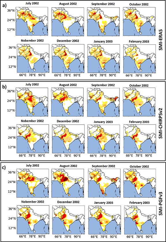
Figure 6. Spatial patterns of agricultural droughts during July 2002 to February 2003 estimated with three different precipitation products: (a) ERA5, (b) CHIRPSv2, and (c) PGFv3.
Download figure:
Standard image High-resolution imageThe impact of the forcing dataset on the spatial pattern of this large event is investigated here by keeping everything constant but the forcing datasets. Figure 6 shows the spatial distribution and evolution of the event estimated with PGFv3, CHIRPSv2 and ERA5 precipitation datasets from July 2002 to February 2003. A recent study by Mishra et al (2018) on drought in India reflects that the 2002 drought occurred in monsoon season (June, July, August and September) in India, it had an areal extent of 33.5% (severe to exceptional drought). In our study we find that in SA, the drought was severe in monsoon season of 2002 and continued until February 2003. Analysis based on all three datasets shows that in monsoon season 18% to 28% of SA was under the 'severe' to 'exceptional' drought condition. We also find that the overall drought pattern produced by different datasets is similar, but there are differences in their areal extent. For example, in August 2002 PGFv3 based output shows 43% area of SA was under drought and 6% area under 'exceptional drought' (see figure 6(c)). Whereas, CHIRPSv2 and ERA5 based output show 35% and 38% under drought respectively and only 1% of the area under 'exceptional drought' (see figures 6(a) and (b)).
4. Conclusion and future direction
Considering the impact of drought in SA, where a large number of people is dependent on rain-fed agriculture, the application of the SA drought monitor (SADM) system has potential to support capacity building and improve policy and practices related to water and agriculture. The SADM serves as an open interactive platform to monitor daily and monthly agricultural drought from regional to local levels at high resolution. The outputs of the SADM are driven using high resolution and near real-time forcing (ERA5) datasets. Since direct observation of soil moisture is not available for SA, such simulation of soil moisture, based on a hydrological model, can help to adopt mitigation and adaptation measures against agricultural drought. The SADM updates the soil moisture maps daily, with a latency of 5 days. The SADM also provides the historical drought maps and the time series plots of the area under drought in SA and has an option for downloading the SMI data.
The comparison of the SMI and SPEI based on CHIRPSv2, ERA5, and PGFv3 precipitation datasets indicates that they have similar temporal distribution; however, in some years (e.g. 1983, 1988, 1990, 1992, 2009 and 2015) there are differences between SMI and SPEI in representing long-lasting soil water deficits. Although, there are years when the SPEI at shorter (4 and 6 months) and longer (9 and 12 months) timescale differ; for example, in 1994, 2006, 2007 and 2010, the 9 and 12 month CHIRPSv2-SPEI show more droughts than the 4 month CHIRPSv2-SPEI and CHIRPSv2-SMI. Additionally, during the wet years (from 1992 to 1998 and from 2007 to 2013) the SMI estimations show more variations than during dry years. An evaluation of model sensitivity with different precipitation datasets shows that precipitation forcings affect the simulated soil moisture. In other words, the precipitation dataset is a fundamental source of predictive uncertainty that should be carefully considered. The comparative analysis of the SMIs estimated with three precipitation products (CHIRPSv2, ERA5 and PGFv3) show an overall similar temporal pattern; however, there are differences in their average area, duration, and magnitude. Furthermore, the difference in the ranking and spatial extent of major drought events is also influenced by the different precipitation products. The drought of 1986–1988 affected 29% of the area based on CHIRPSv2 and 20% of the area based on ERA5 dataset. A detailed investigation of the pre-processing method of various rainfall dataset might help to understand their impact on hydrological model performance. Otherwise, it is difficult to draw any conclusion about which precipitation product is best suited for SA.
The current adaptation of SADM is the initial impetus in application of mHM for drought monitoring of SA, inspired from the German Drought Monitor (www.ufz.de/index.php?en=37937) (Zink et al 2016). There are several fronts in which the SADM could be improved. First, a single model simulation may not be enough for conclusively identifying benchmark drought events (Samaniego et al 2013). Enhancing SADM to a probabilistic drought monitoring based on multiple models and forcing datasets (Turco et al 2020) could be a way forward. Similarly, comprehensive analysis of the impact of agricultural drought on the crop yield will be helpful for the region. Understanding the human influence on water resources; for example, irrigation, reservoir operation and management of trans-boundary rivers is also important for drought management in SA. Further research is needed to incorporate these into the system. Currently, the system does not provide drought forecasts that may help in taking sufficient action. These key issues constitute potential avenues for future upgrades of the system.
Data availability statement
The data that support the findings of this study are available upon reasonable request from the authors.
Acknowledgments
The first author acknowledges that this study was carried out with a Fellowship (2019, ID = BGD1202252IKS) of the Alexander von Humboldt foundation. The set up of the mHM model at a global scale was partly funded by the BMBF project Seasonal water resources management in semi-arid regions: transfer of regionalized global information to practice (SaWaM, project number: 02WGR1421G). We would also like to acknowledge the usage of different data sets: the ERA5 data is available on the Copernicus Climate Change Service (C3S) Climate Data Store: https://cds.climate.copernicus.eu/cdsapp#!/dataset/reanalysis-era5-single-levels?tab=overview. The CHIRPS v2 data set from the Climate Hazards Group (https://chc.ucsb.edu/data/chirps). The Princeton Global Forcings v3.0 (PGFv3) data set is available at https://hydrology.princeton.edu/data.pgf.php. The terrain elevation data was collected from USGS EROS Archive—Digital Elevation—Global Multi-resolution Terrain Elevation Data 2010 (GMTED2010), available at www.usgs.gov/centers/eros/science/usgs-eros-archive-digital-elevation-global-multi-resolution-terrain-elevation. Gridded soil information was obtained from the International Soil Reference and Information Centre (ISRIC, see online at https://soilgrids.org/#!/?layer=ORCDRC_M_sl2_250m#x0026;vector=1). The geological dataset was downloaded from Institute for Biogeochemistry and Marine Chemistry, KlimaCampus, Universitt Hamburg (https://doi.pangaea.de/10.1594/PANGAEA.788537). Leaf area index (LAI) dataset was downloaded from the global land cover facility (GLCF), available at http://iridl.ldeo.columbia.edu/SOURCES/.UMD/.GLCF/.GIMMS/.NDVIg/.global/index.html. The land cover dataset was downloaded from the European Space Agency (ESA), available at http://due.esrin.esa.int/page_globcover.php.
Appendix A.: Definition of drought characteristics
The mean duration (D) of a spatiotemporal drought event indicates the average of the drought duration of every cell in months within a drought event. The mean areal extent (A) is the average area of a region under drought from the onset until the end of the drought event, expressed as a percentage of the total domain. The total magnitude (M) is defined as the spatiotemporal integral of the SMI below the threshold value (SMI  0.2) over those areas affected by the drought (Samaniego et al
2013). Consequently, it is expressed in months times percentage of total domain surface area.
0.2) over those areas affected by the drought (Samaniego et al
2013). Consequently, it is expressed in months times percentage of total domain surface area.
Appendix B.: mHM evaluation
Figure A1 shows a validation of the mHM model for total water storage anomaly (TWSA) and evapotranspiration (ET). The evaluation of TWSA against the Gravity Recovery and Climate Experiment (GRACE) product (Landerer and Swenson 2012) shows moderate to high correlation (r = 0.4–0.8) in Bangladesh, Nepal, Bhutan, and the central and eastern parts of India, but weak correlation in Pakistan, Afghanistan, and north-western India. The evaluation of ET against a gridded FLUXNET product (Jung et al 2011) shows monthly correlations above 0.9 for most of the domain. Moreover, anomaly correlation between ET and the FLUXNET is between 0.5 and 0.7 in most of the areas of western India, Pakistan and Afghanistan. Less correlation is found in the eastern part of the domain.
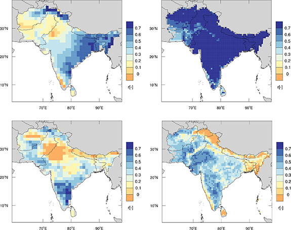
Figure A1. mHM evaluation for (top-left) terrestrial water storage anomaly (TWSA) against GRACE products at 1∘ resolution (2004–2016), (top-right) evapotranspiration (ET) against the FLUXNET gridded product at 0.5∘ resolution (1982–2011) and (bottom-left) anomaly correlation for TWSA and (bottom-right) anomaly correlation for ET.
Download figure:
Standard image High-resolution imageAppendix C.: SPEI estimation
The SPEI is calculated based on the climatic water balance (precipitation minus potential evapotranspiration (PET)) (Vicente-Serrano et al 2010). We estimate the SPEI at a 0.25∘ resolution using all three precipitation datasets (CHIRPSv2, PGFv3 and ERA5 ) and the PET is estimated based on the Hargreaves method (Hargreaves and Samani 1985), where the temperature input is PGFv3. The SPEI is estimated using the non-parametric kernel-based approach (same as the estimation of SMI) developed by Samaniego et al (2013).
Appendix D.: Correlation matrix of SPEI and SMI
The correlation matrix shows correlation coefficients between SMI and SPEI (4, 6, 9 and 12 months) based on three different data sets from 1983 to 2015. For the calculation of the correlation, the PET and soil moisture is first averaged in space over the study domain. In a next step, the SPEIs and SMIs are calculated for the spatial average. Finally, the Pearson correlation coefficient is calculated for the SPEI and SMI. The correlation matrix shows that ERA5-SMI has a significant and positive correlation with PGFv3-SMI (0.88), CHIRPSv2-SMI (0.75), PGFv3-SPEIs (ranges from 0.71 to 0.73) and CHIRPSv2-SPEIs (ranges from 0.63 to 0.72). Whereas CHIRPSv2-SMI has a moderate positive correlation with PGFv3-SMI (0.54) and PGFv3-SPEIs (differ from 0.44 to 0.5) (figure A2).

Figure A2. Correlation matrix of SMI and SPEI (4, 6, 9 and 12 months) for CHIRPSv2, ERA5 and PGFv3 precipitation dataset from 1983 to 2015.
Download figure:
Standard image High-resolution image