

Abstract
Across the globe, recent work examining the state of freshwater resources paints an increasingly dire picture of degraded water quality. However, much of this work either focuses on a small subset of large waterbodies or uses in situ water quality datasets that contain biases in when and where sampling occurred. Using these unrepresentative samples limits our understanding of landscape level changes in aquatic systems. In lakes, overall water clarity provides a strong proxy for water quality because it responds to surrounding atmospheric and terrestrial processes. Here, we use satellite remote sensing of over 14 000 lakes to show that lake water clarity in the U.S. has increased by an average of 0.52 cm yr−1 since 1984. The largest increases occurred prior to 2000 in densely populated catchments and within smaller waterbodies. This is consistent with observed improvements in water quality in U.S. streams and lakes stemming from sweeping environmental reforms in the 1970s and 1980s that prioritized point-source pollution in largely urban areas. The comprehensive, long-term trends presented here emphasize the need for representative sampling of freshwater resources when examining macroscale trends and are consistent with the idea that extensive U.S. freshwater pollution abatement measures have been effective and enduring, at least for point-source pollution controls.
Export citation and abstract BibTeX RIS

Original content from this work may be used under the terms of the Creative Commons Attribution 4.0 license. Any further distribution of this work must maintain attribution to the author(s) and the title of the work, journal citation and DOI.
1. Introduction
Recent large-scale studies of aquatic ecosystems have been facilitated by a growing number of easy to use global [1] and sub-continental [2–4] datasets of field water quality measurements. However, research into one of the largest such datasets [2] suggests that historical field samples tend to be biased towards larger, problematic waterbodies and often lack the temporal continuity necessary for detecting long term trends [5]. Using this unrepresentative data to understand regional to national scale lake dynamics can lead to significantly different results when compared to statistically representative samples [6, 7]. While this problem of representativeness is increasingly acknowledged in sampling efforts (e.g. the U.S. National Lake Assessment; NLA) [8] systematic sampling programs are costly, can have limited temporal resolution and continuity, and require compromise between scientific rigor and logistical practicality [9]. No such sampling program is available at continental scales over multiple decades.
One response to the challenges represented by field studies is to use remote sensing to estimate water quality parameters. Over the past decade, inland water quality remote sensing research has increasingly focused on larger spatial and temporal domains in order to address challenging science questions [10–12]. Here, we use remote sensing to conduct the first multi-decadal, national-scale assessment of U.S. lake water clarity by developing a carefully validated data-driven model that is generalizable across more than three decades for the entire contiguous U.S. We calculate regional summer lake water clarity trends from 1984 to 2018 across nine U.S. ecoregions in two different samples of lakes: a statistically stratified sample (n = 1029 lakes) defined by the 2012 NLA [13] and a large random sample (n = 13 362 lakes) from the National Hydrography Dataset (NHD) [14]. We compare the overarching trends from these remotely sensed estimates to each other and to the entirety of the available in situ data from the Water Quality Portal (WQP) [3] and LAGOS-NE [2], which jointly have over one million field observations of U.S. lake clarity dating back to 1984. In doing so we observe the impact of different sampling approaches and illustrate the biases that exist when using historical field samples to identify long term trends. To complement the ecoregion analysis and compare our work to existing studies focusing on larger lakes [11], we add all U.S. lakes larger than 10 km2 to our NLA and random samples and examine trends in lakes with over 25 years of observations (n = 8897) to identify how lake-specific trends vary with lake size and population density.
2. Materials and methods
2.1. Data processing and acquisition
Figure S1 (available online at stacks.iop.org/ERL/16/055025/mmedia) depicts a summary of the project workflow. Data for model training and validation was derived from a variant of the AquaSat database [15, 16] which combines historical water quality measurements from the WQP [3] and LAGOS-NE [2] with coincident (±1 d) satellite images from the USGS tier 1 surface reflectance collections for Landsat 5, 7, and 8. While the atmospheric corrections used to generate these surface reflectance products were originally developed for terrestrial applications, a growing body of research shows that they can be used to accurately estimate inland water quality parameters and perform on par with water-specific atmospheric correction algorithms [17–19]. Site IDs from AquaSat were spatially joined to lake polygons from NHDPlusV2 [14] (NHD) and then linked to catchment level metrics from the LakeCat database [20]. From the initial AquaSat database, observations were removed if:
- they did not coincide with a lake polygon from NHDPlus V2
- over half of the water pixels within 120 m of the sample site were classified as anything other than high confidence water by the USGS Dynamic Surface Water Extent water mask [21]
- the Landsat scene contained over 50% cloud cover
- one or more Landsat bands was beyond a reasonable reflectance for water (0–0.2)
- the Fmask [22] indicated the presence of clouds, cloud shadows, or ice over the sample site
- the observation was impacted by topographic shadow
- recorded field water clarity (measured as Secchi disk depth) was <0.1 m or >10 m (the limits used for the NLA field sampling).
- two identical clarity observations occurred on the same day within the same lake as a result of duplication between WQP and LAGOS-NE (WQP observations were kept while LAGOS-NE observations were removed in these circumstances)
Similarly, reflectance values for analyzing national clarity trends were calculated using the same filters and methodology described above using the lake center as the sample point and taking the median value of high confidence water pixels within 120 m for all study lakes. As an additional test, the predictions using lake center median values were compared with predictions using whole lake median values for the 2012 NLA lake sample. The two sets of predictions showed strong agreement (R2 = 0.95, figure S2), so lake centers were used for consistency with AquaSat's point based method. All reflectance values were extracted from Google Earth Engine [23] for the three samples of interest within the study: the statistically stratified NLA 2012 sample (n = 1038), a large random sample of 2000 lakes per ecoregion (n = 18 000), and all lakes greater than 10 km2 (n = 1170).
Each subsample contained a portion of lakes that were ultimately removed through the quality control measures described above. Spot checking of the removed waterbodies revealed that the most common cause for removal was lack of Landsat visible pure water pixels caused by either irregular waterbody shape (long and narrow), surface vegetation on the waterbody, overhanging vegetation along the shoreline, or a misclassification of a lake within NHD. Removal of these waterbodies led to total lake counts of 1029 for the NLA sample, 13 362 for the random sample, and 1105 for lakes over 10 km2 (for a total of 14 971 unique lakes). While conservative, this filtering approach ensured minimal error from mixed pixels, sun glint, and surrounding adjacency effects from nearby land.
Reflectance values from the differing Landsat sensors were normalized following Gardner et al [24]. For each satellite pair (Landsat 5/7 and Landsat 7/8), the reflectance values observed over the entirety of the NLA sample of lakes were first filtered to coincident time periods when both sensors were active (1999–2012 for Landsat 5 and 7 and 2013–2018 for Landsat 7 and 8). We assume that the distribution of collected reflectance values for a given band should be identical given a sufficient number of observations over the same array of targets regardless of sensor. Based on this assumption, we calculated the 1st–99th reflectance percentiles for each sensor/band during periods of coincident satellite activity. Since Landsat 7 spans the time periods of both Landsat 5 and Landsat 8, each band in 5 and 8 was corrected to Landsat 7 values through a 2nd order polynomial regression of the 1st–99th percentiles of reflectance values between the two sensors for the overlapping time period (figure S3). The resulting regression equations were then applied to all Landsat 5 and 8 values within AquaSat as well as for all the included study lakes. Ultimately, applying these corrections to the reflectance values reduced the final model mean absolute error by 0.2 m, suggesting that standardizing the reflectance values between sensors successfully reduced errors from sensor differences.
Application of the above quality control measures for AquaSat resulted in a model training and testing database of 250 760 observations of Secchi Disk depth, associated Landsat reflectance, and site specific lake and catchment properties for an optically diverse sample of waterbodies across the United States dating back to 1984 (figure S4). Reflectance values for specific bands and band ratios within the training dataset were analyzed for correlations with atmospheric optical depth derived from the MERRA2 reanalysis data [25]. Correlations were examined both over the entire study period and between 1991 and 1993, when aerosol optical depth values were particularly high due to the eruption of Mt. Pinatubo. Optical parameters that showed the least correlation to atmospheric optical depth (r < 0.15 during 1992 and 1993 and r < 0.1 for the study period) were then chosen for inclusion in the modelling pipeline. These included Blue/Green and Nir/Red ratios and the dominant wavelength as described by Wang et al [26].
Of the non-optical parameters from the LakeCat database, we included those that could impact water clarity and were mostly static over time (table S1). Static 2006 values for catchment level percent impervious surfaces, percent urban landcover, percent forested landcover, percent cropland, and percent wetland landcover were included despite potentially being unrepresentative of the entire study period in some catchments. These variables were deemed important based on existing research [27, 28], domain expertise, and various preliminary empirical tests of feature importance, and therefore were included in the modelling pipeline. All lake and landscape-level variables were rounded to the nearest tenth or whole number, depending on the variable scale, in order to prevent certain variables from acting as location identifiers and to avoid overfitting during model training. This initial reduction in the feature space of the training dataset resulted in three optical variables and 27 static lake/landscape variables for each AquaSat matchup observation.
2.2. Model development and validation
Non-parametric, supervised machine learning algorithms are increasingly popular within the remote sensing community due to their robustness, ease of use, and relatively low computational requirements [29]. Among these algorithms, extreme gradient boosting (Xgboost) has been shown to outperform similar non-parametric classification and regression schemes for urban land cover classification [30], determining aerosol optical depth [31], and modeling solar radiation [32]. Xgboost classifiers are ensemble models that combine a suite of 'weak' classifiers in order to minimize overall error. Within each iteration, estimates with large errors from the previous iteration are weighted in order to force the model to maximize its performance on the most challenging calibration data. The iterations are additive, meaning that the final model is the sum of the previously weighted regressions.
Here, we use the generalized linear module of Xgboost as it was found to outperform the tree based module for low values of water clarity. This implementation of Xgboost creates a generalized linear model using elastic net regularization [33] and coordinate descent optimization [34]. To better understand the structure of the final model, as well as the influence of each input feature on model predictions, we calculated the feature importance and accumulated local effects (ALEs) [35] for all model inputs (figure S5). ALE values represent the average marginal impact of a feature on final predictions as the feature value increases or decreases along a localized window of values. Examining ALE values is an effective method for interpreting machine learning models that are otherwise opaque in their structure (i.e. black boxes) [36].
In order to avoid model overfitting and limit the final number of input variables, we incorporated forward feature selection (FFS) [37] with target oriented leave-location-leave-time out cross validation (LLLTO-CV) [38] into our Xgboost model development. FFS and LLLTO-CV effectively reduce overfitting by cross-validating the model on locations and times not used for model training and removing variables with high spatial or temporal correlations with observed clarity. We set aside 20% of the training dataset (n = 50 153) to use for post-development model testing and trained our initial model with the remaining 80% (n = 200 607) using FFS and LLLTO-CV. This process reduced the overall number of input variables from 30 to 11 (three optical properties and eight static lake/landscape variables) (table S1). Finally, the hyperparameters of the model were tuned using a grid search approach with conservative hyperparameter values.
2.3. Annual lake water clarity predictions
Lake observations downloaded from Google Earth Engine were limited to those between May and September in order to remove the influence of snow and ice while maximizing the number of cloud free images captured. For any given lake and year, the median of all cloud free predictions was taken as representative of summer lake clarity. These summer clarity predictions were then averaged across the nine ecoregions defined within the NLA to generate estimates of annual regional water clarity. For the NLA sample of lakes, this process led to an average of 883 observations spread across 103 lakes being averaged for each regional estimate of summer water clarity. The NLA provides weights for lakes used in analyses at the state and national scale; however, no ecoregion scale weights are provided, and therefore regional means calculated here represent the unweighted regional means of the 2012 NLA sample lakes.
Model error was propagated into the mean regional estimates through 1000 iterations of bootstrap sampling. Within each iteration, annual lake median values within each region were sampled with replacement, and the new subsample was used to calculate the annual mean for the region. This bootstrapping procedure effectively propagates a different amount of model noise into each estimate of mean summer clarity by incorporating a different sample of lakes into each iteration of the regional estimate. This resampling results in a distribution of 1000 estimates of clarity for each year/region. We take the mean ± standard deviation of these distributions to generate 90% confidence bounds for each annual estimate of clarity.
In order to analyze overarching regional trends, we calculated Thiel–Sen slopes for each of the generated time series based on the mean of the bootstrap sampling procedure. Thiel–Sen slope is a nonparametric measure of the magnitude of monotonic trends that is insensitive to outliers within the dataset [39]. It determines overall trends by calculating slopes between each pair of points in a time series and then taking the median of all slopes. It is often used in conjunction with Mann–Kendall trend analysis to quantify the more binary Mann–Kendall tau statistic [40]. The trends presented here are based on the full remote sensing time series; however, we also calculated trends excluding the years in which atmospheric optical depth was potentially impacted by the Mt. Pinatubo eruption (1991–1993). Overall trends using the filtered timeseries showed only minor differences from the full-time series (figure S6) indicating that the reported patterns observed here are not artefacts of the abnormal atmospheric conditions in the early 1990s. Trends for the field data were analyzed using the same method as the remote sensing predictions by first taking the summer median of each sampling point, averaging the median values by year/region, and calculating Thiel–Sen slopes from the resulting regional estimates.
Finally, we identified lakes with more than 25 years of observations to conduct lake-scale analysis (n = 8897). We calculated Thiel–Sen slopes for each individual time series of median summer clarity to examine the distribution of trends at the lake scale. Individual lake trends were binned by lake size and catchment population density to analyze the impact of these lake characteristics on overall clarity trends. The resulting distributions across size classes and catchment population density showed longer tails towards positive trends and were therefore analyzed using non-parametric Mann–Whitney tests rather than the more common parametric t-test. While we did not explicitly propagate model error into these individual lake time series, we attempt to reduce the impact of model noise by examining distributions rather than individual lakes and calculating the median trend for each binned distribution.
3. Results
3.1. Model validation
Validation of our data-driven remote sensing model (figures 1 and S7) indicates that it performs on par with existing regional remote sensing models developed using either traditional regression methods or semi-analytical modelling [12, 41, 42]. However, unlike previous regional models that are only applicable to a specific scene, sensor, or area, the model presented here is generalizable for over three decades for the entire contiguous United States. Model error was calculated using the hold-out data (n = 50 153) not used in model training. Error metrics were calculated at the observation level as well as at the aggregated ecoregion level used in the final analysis. Examination of the model residuals shows a consistent normal distribution over time. This is important both because it reaffirms the sensor correction procedure described above and because it leads to more accurate regional estimates, as over and underpredictions cancel each other out. Observation level error metrics for the final model include a mean absolute error of 0.71 m (mape = 38%) and bias of <0.01 m. Regional/annually aggregated error metrics include a mean absolute error of 0.25 m (mape = 14%) and a bias of −0.02 m. The distributions of estimates generated through the bootstrap sampling procedure have an average standard deviation of 0.09 m around the mean estimate. As each re-sampling propagates varying amounts of model error into the final mean annual value for a region, this low standard deviation suggests that the bootstrapping procedure likely further reduces the uncertainty of our annual regional estimates.
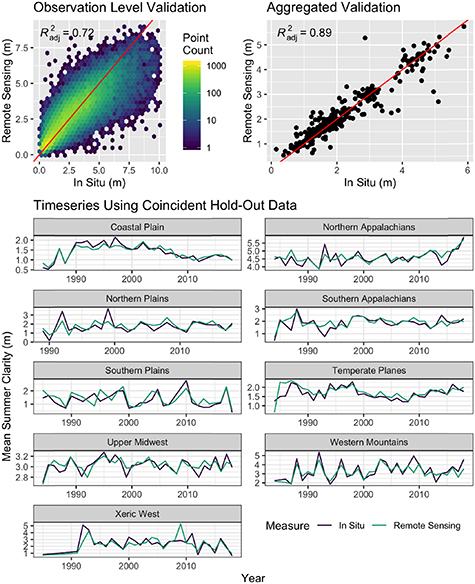
Figure 1. Model validation based on hold-out data not used in model development. Clockwise from the upper left: point based model performance, model performance aggregated by year and region, and regional timeseries of aggregated validation. Note that the time series shown only include hold-out estimates coincident with field measurements used for validation and do not represent the final time series of the study. They are provided to illustrate that the validation captures regional temporal patterns seen in the field data.
Download figure:
Standard image High-resolution imageFeature importance, measured as gain (i.e. the improvement in accuracy when a given feature is included), shows that optical variables, especially the dominant wavelength, contribute the most predictive capability to the model (figure S5). To further validate the contribution of optical variables to the model, we validated a second, purely optical model on the same training and testing data which resulted in an RMSE of 1.3 m. The purely optical model was able to explain 50% of the total variance (R2) within the validation dataset compared to 72% from the combined landscape model. This difference indicates that the optical parameters contributed up to 70% (0.50/0.72) of the explained variance within the final combined landscape model, with the static lake and landscape variable characteristics contributing at least 30%. The calculation of ALE values provides additional detail on the underlying structure of the model as well as evidence that the model is capturing many of the physical relationships we would expect. For example, we see that as the dominant wavelength of an observation moves from 475 nm (within the blue spectrum) to 560 nm (within the green spectrum) the impact on clarity predictions goes from a 50 cm increase to a 75 cm decrease. This difference likely captures decreased clarity as algae and suspended sediment increases.
Model performance was also broken down by lake size, satellite, data source, and time to ensure that predicted trends were not artefacts of lake or sensor characteristics (figure S7). While variations in model fit across lake sizes, sensors, and data sources are nominal, the validation did show a slight increase in bias over time, with clarity in earlier years being slightly overpredicted on average and clarity in later years being slightly underpredicted. However, if anything, this small change in bias over time makes our trend predictions conservative as later years are generally underpredicted. We included a breakdown by data source because LAGOS-NE field measurements are all geolocated to lake center points while WQP uses explicit sampling site coordinates [15]. For observations recorded in both, we deferred to WQP because of the spatial specificity. However, validation results from both datasets show strong agreement, likely because the vast majority of lakes are small enough that there is minimal variation between lake center points and nearby sampling locations. This similarity also supports the above stated decision to predict clarity based on median center point reflectance values rather than median whole lake reflectance values.
As an additional check, we conducted two comparisons of model performance against known benchmarks in the field. First, we compared our regional estimates of lake water clarity to those of the 2007 and 2012 NLAs and found strong agreement between the reported field values and our model predictions (mape = 17.7%) (figure S8). Second, we generated mean summer predictions for the individual lakes included in LakeBrowser [12], a well-validated water clarity remote sensing project focused on over 10 000 lakes in Minnesota (https://lakes.rs.umn.edu/). Comparison of the predictions from the two modelling approaches show agreement when comparing annual estimates at the ecoregion level used by LakeBrowser (R2 = 0.82) and when compared to field data from the WQP and LAGOS-NE (figure S9).
3.2. Trends in U.S. lake water clarity
Time series generated for the NLA sample of lakes show that, on average, water clarity in U.S. lakes increased at a rate of 0.52 cm yr−1 from 1984 to 2018. Seven of the nine NLA ecoregions show significant positive trends (p < 0.05) that varied from 0.23 cm yr−1 (p = 0.040) in the Coastal Plains to 1.00 cm yr−1 (p < 1e−5) in the Northern Appalachians (figure 2). Significant trends were absent in the Southern Appalachian and Southern Plains regions, but no region had a significant decline in clarity. All regions with significant trends show clarity shifts throughout the study period that are greater in magnitude than their mean confidence interval.

Figure 2. Regional modelled trends in water clarity for the statistically stratified sample of NLA lakes that are Landsat visible and a large random sample of Landsat visible lakes. Trends and their associated confidence intervals represent the mean and standard deviation of values calculated through 1000 iterations of bootstrap sampling of the NLA and random sample lakes respectively. Points on maps represent individual lakes included in the sample. Asterisks indicate significance levels of trends determined by Thiel–Sen slopes at 90% (*), 95% (**), and 99% (***) confidence levels for the NLA sample of lakes.
Download figure:
Standard image High-resolution imageInterannual variations in percent clarity change between ecoregions are significantly correlated (p < 0.05) in 24 of the 36 (67%) possible region pair combinations (figure S10). Additionally, during 29% (n = 10) of the observed years, at least eight of the nine ecoregions showed synchronous increases or decreases in clarity compared to the previous year. While some of these years line up with discrete events (e.g. 1987 was heavily impacted by the Pacific Decadal Oscillation), ascribing this synchrony to specific climatological or anthropogenic drivers is difficult due to the multiscale controls on lake water clarity [27, 43]. However, the scale of the changes suggests that drivers of water clarity function at national scales for at least some parts of the study period.
3.3. Impacts of lake size and population
Recent studies of large-scale drivers of inland water quality suggest both that (a) a variety of anthropogenic and climate forcings are leading to an increase in algal blooms and concomitant decreases in water clarity in many lakes [11, 44], and that (b) nutrient loading of U.S. rivers, particularly near urban areas, is decreasing [45, 46], a trend that should translate to decreased algal growth in downstream waters, particularly if these receiving systems have relatively short mean water residence times or are isolated from non-point sources of nutrient inputs [47, 48]. These contradictory narratives may reflect limited use of representative samples at large spatial scales, with most studies systematically under-sampling smaller waterbodies despite their numerical dominance and ecological significance [49].
To better compare our analysis to previous work focusing on larger lakes and river systems, we generated annual water clarity time series for all U.S. lakes larger than 10 km2 (n = 1105) in addition to our NLA and random samples to create a full dataset of 14 971 unique lakes. From this sample, we selected only those lakes with at least 25 years of cloud-free remote sensing observations (nlakes = 8897 lakes, nobservations = 2 727 021) and binned them by size class (<1, 1–10, 10–100, and >100 km2) and catchment population density (20% quantiles) to compare how trends differed by lake size and examine potential links to improving stream water quality in urban areas. The resulting distributions of trends show that the most significant clarity improvements are occurring in smaller waterbodies and in densely populated areas (figure 3). Lake size and population density are not significantly correlated, nor are these results related to differences between natural lakes and reservoirs, which show no significant difference in their distribution of trends (p = 0.69). For lake size, median trends for lakes in the smallest to largest size classes are 0.28, 0.19, 0.08, and 0.02 cm yr−1, respectively, with all but the last class significant at a 99% confidence level. Trends for lakes in catchments within the lowest population density quintile (20%) were approximately four times smaller than for lakes in the most urban upper quintile (p = 2.2e−16). Given these trends and the important controls of population density and lake size, research focusing primarily on large lakes may accurately find that water clarity is not increasing. However, the more systematic analysis presented here provides a more complex story in which clarity dynamics are dependent on lake-specific limnological and geographic attributes.

Figure 3. Distribution of modelled trends in lakes with greater than 25 years of observations by (left) lake size class (<1 km2, n = 7339; 1–10 km2, n = 509; 10–100 km2, n = 925; >100 km2, n = 124) and (right) 2010 catchment population density quantiles. Actual values for quintiles in terms of people per km2: [0–1], (1–3], (3–11], (11–43], (43, 3970]. Y-axis limits set to −5 to 5 for visualization.
Download figure:
Standard image High-resolution image3.4. Sampling impact on patterns of water clarity
To examine the effect of lake sampling on observed patterns in water clarity, we replicated our NLA analysis using: (a) remote sensing estimates for a large random sample of lakes (n = 13 362, figure 2), and (b) the entirety of field data from both LAGOS-NE and WQP, two of the largest national field databases of water quality in the U.S (n = 1 296 659 observations between 1984 and 2018). Results of this comparison show that the NLA sample of lakes accurately reflects temporal patterns of lake clarity across ecoregions compared to a random sample, with some minor geographical exceptions (figure 2). Regardless of these differences, regional temporal patterns in water clarity are highly correlated between the NLA and random samples, with Pearson's Correlation Coefficients ranging from 0.55 (p = 5.4e−4) in the Southern Plains to 0.91 in the Upper Midwest (p = 1.0e−5). These high correlations between samples suggest that the NLA sample is representative of a larger random sample of lakes and that observed trends are insensitive to lake sampling given a large enough sample size and regular sampling intervals.
Conversely, comparison of the remotely sensed NLA and large random samples to historical field observations from LAGOS-NE and WQP reveals substantial discrepancies in overall trends (figure 4). Time series of historical regional clarity calculated with the full set of field data lack significant correlations (p < 0.01) with the time series from the NLA sample in seven of the nine study regions. Slopes differ by orders of magnitude from the closely matched random and NLA samples, in some cases with significant trends in the opposite direction. These results emphasize that conducting an identical analysis with spatiotemporally inconsistent and potentially ad hoc field sampling leads to substantially different trends in water clarity compared to the same analysis using representatively sampled remote sensing estimates.

Figure 4. Differences in observed ecoregion trends when conducting the analysis with all the in situ samples from the WQP/LAGOS-NE and the modelling results from the NLA lake sample and a large random sample. Asterisks indicate significance levels of trends determined by Thiel–Sen slopes at 90% (*), 95% (**), and 99% (***) confidence levels.
Download figure:
Standard image High-resolution image
4. Discussion
Our analysis of long-term trends in lake water clarity across the United States highlights that:
- (a)Overall clarity in U.S. lakes increased between 1984 and 2018. This increase was concentrated largely in lakes smaller than 10 km2 and in more urban areas.
- (b)A systematic understanding of national patterns in lake water clarity requires a representative sample of lakes. These macrosystem-level patterns are not reflected in aggregated historical field data.
By applying our model across both the NLA sample of lakes and a larger random sample, we successfully capture long-term patterns in U.S. lake water clarity that are unobservable in historic and contemporary field sampling efforts. The NLA represents the current best-practice in large scale field monitoring across the U.S.; however, we show that lake clarity nationally has distinct temporal patterns that are not fully captured with the 5 year return period of the NLA field sampling efforts. High correlations between trends observed with different lake samples, high correlations in time series among regions, and periods of uniform change at the national scale all point to the influence of one or more drivers of lake water clarity operating at a national scale or larger. We examined relationships between observed water clarity patterns and potential forcing variables (temperature, precipitation, sulfate deposition, and the Pacific Decadal Oscillation, figure S11) and found that the regional impacts of these correlations varied, likely due to complex, cross-scale interactions that lead to variable regional influences as different drivers interact with each other [3, 27, 43]. However, while more difficult to quantify, the period analyzed here begins directly after a round of sweeping environmental legislation in the 1970s and 1980s. These major national level policies include the Clean Water Act (CWA 1972; amended 1977 and 1987), the National Environmental Policy Act (NEPA 1969), the Clean Air Act (CAA 1963, amended 1965, 1966, 1967, 1969, 1970, 1977, 1990), the Safe Water Drinking Act (SWDA 1974, amended 1986,1996), and the Endangered Species Act (ESA 1973), all of which targeted freshwater resources and habitat to varying extents.
Our results are consistent with recent studies showing regional [50, 51] and national [45, 46] improvements to U.S. streams and rivers [45, 46, 50, 51] and lakes [46] directly attributable to the CWA. Specifically, they show declining nutrient concentrations in urban areas caused by reductions in point source pollution and improved stormwater management emphasized by the CWA. Although agricultural streams have not undergone significant changes in nutrient loads, they have shown declines in suspended sediments, consistent with improved sediment management practices [45]. These recorded improvements in streams and rivers provide a mechanism for increasing lake water clarity, as changes in fluvial systems often equate to changes in sediment and nutrient inputs to lakes [52]. This argument assumes that the observed improvements in clarity can be attributed to declining suspended sediment and nutrient concentrations rather than the other contributor to water clarity—'colored' dissolved organic matter (cDOM) because where cDOM patterns exist in lakes, they are predominantly positive [53] and therefore not contributing to increases in clarity.
Evaluating long-term nutrient dynamics is more challenging because of limitations in data availability over the period of study at the national scale. An analysis of the 17-state region represented by the LAGOS database revealed that total nitrogen decreased while total phosphorus concentrations have neither decreased nor increased in the vast majority of lakes sampled during summer months between 1990 and 2013 [54]. While this nutrient decrease alone potentially contributed to increased lake clarity in nitrogen-limited waterbodies, the study lacks lake water quality data that corresponds to the period of greatest change observed in streams, which was steepest from 1982 to 1992 within urban areas [45]. The diminishing improvements in stream water quality after this period are likely because investment in municipal and industrial water pollution control efforts began to gradually taper off in the mid-1990s [55]. Even allowing for a delay in water quality response to phosphorus reductions [47], these funding patterns are consistent with the greatest gains in water clarity occurring over the first two decades of the CWA within lakes in densely settled areas and smaller waterbodies that tend to be more responsive to management activities because of their shorter average water residence times. Our results support this conclusion, with smaller lakes showing over three times the median increase in clarity than larger lakes (p = 4.7e−8), with lakes in catchments with higher population density showing over four times the median increase in clarity than lakes in low population density catchments (p = 2.2e−16) (figure 3), and a slowdown of clarity improvements after 2000 due to diminishing returns of reduced point source pollution. This slowdown was likely exacerbated due to difficulties reducing nonpoint sources of pollution, particularly in some regions of the country where changes in the precipitation regime are exacerbating nutrient loading to surface waters [56].
Comparison of observed trends across the NLA sample of lakes, a large random sample, and historical field records provides both empirical support for the representativeness of the NLA and evidence for the shortcomings of relying solely on potentially biased historical field samples for systematic monitoring of freshwater resources. Examining trends at the lake and regional level highlights the potential for an unrepresentative sample of lakes to inaccurately depict system-wide patterns. Specifically, when we restrict analysis to larger waterbodies, we find only nominal change in U.S. lake clarity, but the more inclusive analysis presented here suggests that overall lake water clarity within the United States has increased over the past 35 years. While this is the first study of trends in lake water clarity at a national scale, it extends regional studies throughout the northeast that have found water quality in lakes is either largely stable or improving [54, 57–59], as well as work in China and Sweden indicating that national management policies are decreasing eutrophication rates [4, 60, 61]. While more work is required to understand the multiscale drivers of water clarity, the results presented here bring us closer to realizing research goals dating back more than 20 years emphasizing that representative sampling is required for effective monitoring of freshwater resources [6, 7].
Acknowledgment
We would like to thank the reviewers that contributed feedback to this manuscript.
Data availability
Data used for this paper come from LAGOS-NE (doi: 10.6073/pasta/0c23a789232ab4f92107e26f70a7d8ef), LakeCAT (ftp://newftp.epa.gov/EPADataCommons/ORD/NHDPlusLandscapeAttributes/LakeCat/FinalTables/), NHDPlusV2 (www.epa.gov/waterdata/nhdplus-national-data), and the Water Quality Portal (www.waterqualitydata.us/portal/).
The data that support the findings of this study are openly available at the following URL/DOI: https://doi.org/10.6084/m9.figshare.12227273.v2.
Code availability
All code for the analysis can be found at https://github.com/SimonTopp/USLakeClarityTrendr.
Author contributions
S N T conducted modelling, data analysis, and manuscript preparation. S N T, T M P, M R V R, and X Y contributed to study design. E H S and C G G contributed limnology and remote sensing expertise respectively. All authors contributed significant manuscript feedback and edits.
Conflict of interest
The authors declare no conflicts of interest in regards to this manuscript.
Funding
Funding for this work came from NASA NESSF Grant 80NSSC18K1398. The contributions from EHS were supported by the National Science Foundation Grant EF-1685534.