

Abstract
The global electric circuit (GEC) is a unique atmospheric system driven by the global distribution of thunderstorms and electrified shower clouds. The GEC unites electric fields and currents in the entire atmosphere and is characterized by the permanent production and dissipation of huge amounts of electrical energy. In this study, aimed at investigating the links between the GEC and El Niño—Southern Oscillation (ENSO), the GEC variability during 2008–2018 is simulated on the basis of reanalysis meteorological data using the Weather Research and Forecasting model and a parameterization of the ionospheric potential (IP), which is a natural measure of the GEC intensity. Modelling shows that strong El Niño and La Niña events influence the global distribution of electrified clouds over the Earth's surface, thereby consistently affecting the shape of the diurnal variation of the GEC. Further analysis shows that anomalies in the Niño 3.4 sea surface temperature, which characterize the ENSO phase, and anomalies in the relative IP are positively correlated at 9:00–15:00 UTC and negatively correlated at 18:00–23:00 UTC. This correspondence between ENSO and the GEC is most prominent at 13:00 UTC and 21:00 UTC, and most pronounced anomalies in the relative IP around these hours are precisely associated with strong El Niño and La Niña events. In particular, during strong El Niños the relative IP is larger than usual around 13:00 UTC and smaller than usual around 21:00 UTC, whereas during strong La Niñas it behaves oppositely.
Export citation and abstract BibTeX RIS

Original content from this work may be used under the terms of the Creative Commons Attribution 4.0 license. Any further distribution of this work must maintain attribution to the author(s) and the title of the work, journal citation and DOI.
1. Introduction
It has long been known that the fair-weather electric field at the Earth's surface looks nearly the same at different locations around the globe, when shown as a function of universal time (the so-called Carnegie curve; see Harrison 2013). Following Wilson's hypothesis (Wilson 1921, 1924), this observation is generally explained by linking the Carnegie curve to the diurnal cycles of thunderstorms and convection on global scales (Whipple and Scrase 1936): it is thought that thunderstorms and electrified shower clouds in general contribute to what is known as the global electric circuit (GEC) and thus determine electric field values in the entire Earth's atmosphere (this concept is often called direct current global circuit, to distinguish it from the so-called alternating current circuit; see Rycroft et al 2000, Williams 2009). The GEC is driven by charge separation inside electrified clouds; the current generally flows upwards towards the ionosphere in the regions occupied by such clouds and flows downwards to the Earth in fair-weather regions. The circuit is completed by the highly conducting (and, by inference, nearly equipotential) Earth and ionosphere; the potential of the latter relative to the former is called the ionospheric potential (IP; Markson 1986, 2007).
However, it was only recently that parameterizations able to simulate the Carnegie curve with weather forecasting and climate models have been suggested (Mareev and Volodin 2014, Lucas et al 2015, Ilin et al 2020). These parameterizations made it possible to (a) provide a firm theoretical basis for Wilson's hypothesis, (b) identify and analyse specific mechanisms of the influence of meteorological factors on the Earth's electrical environment and (c) allow the forecasting of the electrical state of the atmosphere. Recent research has further emphasized the role of the GEC as a crucial component of the Earth system, playing an important part in the interaction of geospheres and linking between space weather and weather on Earth (Rycroft et al 2000, 2008, Tinsley 2008, Williams 2009).
The El Niño—Southern Oscillation (ENSO) is the largest cause of climate variations on Earth after the seasonal cycle of summer and winter. The ENSO cycle is made up of a warm phase (El Niño) and a cold phase (La Niña), when the sea surface temperatures (SSTs) in the central and eastern equatorial Pacific Ocean heat/cool by a few degrees for 12–18 months respectively. This large change in the Earth's climate has major impacts on global temperature patterns (Tsonis et al 2005), global rainfall patterns (Villafuerte and Matsumoto 2015), agriculture and economic output (Adams et al 1999) and even public health (Kovats et al 2003).
The influence of ENSO on the Earth's electrical environment, including the GEC, has been discussed in a number of studies (their review can be found in Williams and Mareev 2014, section 9). However, nearly all of them considered only the effect of ENSO on lightning activity by analysing empirical data of correlations between ENSO indices and some electrical characteristic—usually the number of flashes per unit area in different parts of the globe (Williams 1992, Sátori and Zieger 1999, Goodman et al 2000, Hamid et al 2001, Price and Federmesser 2006, Yoshida et al 2007, Chronis et al 2008, Price 2009, Sátori et al 2009, Kumar and Kamra 2012). The only known paper considering links between El Niño and the surface electric field is the one by Harrison et al (2011), who obtained a positive correlation between the ENSO cycle and the mean fair-weather potential gradient measured at the Earth's surface in December.
There presently does not exist an adequate set of experimental data which would make possible a detailed study of the relationships between ENSO and atmospheric electricity. Notwithstanding that, we can investigate this relationship using models of atmospheric dynamics, which allow both calculating ENSO indices and estimating the electrical parameters. From a theoretical perspective, it is easier to measure the GEC intensity by the IP rather than by the surface electric field, since the former must have the same relative diurnal variation determined by the dynamics of convection (Markson 1986) but is not influenced by local factors such as aerosols. In a sense, one can say that the IP is a unique geoelectric index that allows one to naturally characterize the state of the Earth's climate system. In this paper we investigate the influence of ENSO on the temporal variations of the GEC, simulating atmospheric dynamics on the basis of the data of meteorological observations and using the IP for quantitative analysis.
2. Parameterization of the IP and simulation of the GEC
The current network of the GEC is maintained by electrified clouds, which are for the most part characterized by deep convection. Once we know the state of the atmosphere, we can estimate the IP on the basis of information about convective activity (Mareev and Volodin 2014). To simulate atmospheric dynamics for this study, we used the Weather Research and Forecasting model (WRF; see Skamarock et al
2008, Powers et al
2017) running globally on a  latitude-longitude grid with 51 altitude levels. Initializing the model with meteorological reanalysis data (National Centers for Environmental Prediction, National Weather Service, NOAA and US Department of Commerce 2000), we simulated atmospheric dynamics on every third day during the years 2008–2018 (technical details of the simulation are given in the supplementary information (available online at stacks.iop.org/ERL/16/044025/mmedia)).
We use the following parameterization of the IP, suggested by Slyunyaev et al (2019). Let Si
be the area covered by the ith model grid column. We denote the total amount of precipitable water stored in this column by Wi
and the amount of precipitation in this column totalled over a symmetric 2 h interval by Pi
. We approximate the lower and upper boundaries of the mixed phase region in this column,  and
and  , by the heights of the 0 ∘C and −38 ∘C isotherms, and we denote by εi
the maximum convective available potential energy (CAPE) averaged over the same column. Then the IP V can be estimated in terms of these variables using the equation
, by the heights of the 0 ∘C and −38 ∘C isotherms, and we denote by εi
the maximum convective available potential energy (CAPE) averaged over the same column. Then the IP V can be estimated in terms of these variables using the equation
where the sum is taken over all grid columns, j0 is the characteristic value of the charge separation current density inside electrified clouds, σ0 is the average conductivity at the Earth's surface, H is the average scale height for the conductivity,  is the total area of the Earth's surface and ε0 is a threshold CAPE value, assumed to be 1 kJ kg−1.
The two main ideas behind this parameterization are cutting off the grid columns with weak convective activity (hence the last factor in the formula) and estimating the area covered by electrified clouds (which alone serve as GEC generators) in each column from the amount of precipitation (hence the factor  ). Further discussion of these assumptions and a derivation of formula (1) from fundamental equations for the electric potential can be found in Ilin et al (2020). In specific calculations we use 6 km for the value of H, while the exact values of j0 and σ0 do not matter, for we always focus on relative changes in V.
Parameterization (1) enables us to simulate the diurnal variation of the GEC by averaging the values of the IP over a large number of days and employing certain regularization procedures, described in the supplementary information.
3. Influence of El Niño and La Niña events on the GEC
It is known that the approach to simulating the IP that we use in this study allows one to faithfully reproduce the shape of the Carnegie curve, but tends to underestimate its peak-to-peak amplitude owing to the fact that it is difficult to single out electrified clouds in large-scale models of atmospheric dynamics (Slyunyaev et al 2019). At the same time the agreement is much better (with a correlation coefficient about 0.98) during Northern Hemisphere winters (see Ilin et al 2020), which are most important for studying the effects of ENSO; in addition, systematic errors in our estimates of contributions from various regions should not substantially influence general trends in the year-to-year dynamics of the Carnegie curve. These considerations justify using theoretical modelling to study the influence of ENSO on atmospheric electricity.
3.1. Diurnal variation of the GEC at the peak of a super El Niño
In terms of ENSO, the years 2008–2018, for which we simulated the atmospheric dynamics, were characterized, in particular, by a very strong super El Niño event in 2015–2016. Figure 1 compares the relative diurnal variation of the IP in the 5 month period around December, calculated on the basis of all the data for 2008–2018 (blue solid line), with its counterpart for the same 5 month period around December 2015 (purple solid line), at the peak of this El Niño (in other words, the purple curve is based on averaging over October 2015–February 2016, while the blue curve is based on averaging over all Octobers, Novembers, Decembers, Januaries and Februaries that occurred during 2008–2018). It is easy to see that the graph in the case of the super El Niño is essentially different from the long-term average; in particular, the relative IP is clearly above the mean for the time interval of 7:00–14:00 UTC and below it at 16:00–23:00 UTC. To make this observation more precise, in the same figure we show by dotted lines the same graphs plus and minus one standard error.
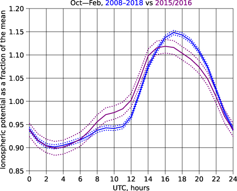
Figure 1. Diurnal variation of the ionospheric potential in the 5 month period around December (October–February) on average (on the basis of the data for 2008–2018; blue solid line) and during the super El Niño of 2015–2016 (on the basis of the data for 2015/2016 alone; purple solid line). The values of the ionospheric potential are given as fractions of the respective diurnal means. Dotted lines show diurnal variations plus and minus one standard error (for more details on calculating standard errors in this study, see supplementary information).
Download figure:
Standard image High-resolution image3.2. Diurnal variation of the GEC during lesser ENSO events
Other El Niño and La Niña events that occurred during 2008–2018 were less pronounced than the El Niño of 2015–2016. They include strong La Niña events in 2010–2012 with the main peak at the end of 2010 and a secondary peak at the end of 2011 and a pronounced El Niño event in 2009–2010. Figure 2 shows the counterparts of figure 1 for all October–February periods during 2008–2018. Unlike the situation in the case of the super El Niño of 2015–2016, plots for other years do not show such a pronounced deviation from the long-term average, and one standard error wide bands around the two plots usually overlap. However, we can still identify lesser aberrations due to the 2010–2012 La Niñas and 2009–2010 El Niño. The effect of the 2009–2010 El Niño is somewhat similar to the effect of the 2015–2016 El Niño, albeit much subtler; the relative IP is above the mean at 10:00–17:00 UTC and below the mean at 20:00–4:00 UTC. The effect of La Niñas in 2010–2011 and 2011–2012 manifests itself in the relative IP being above the long-term mean at about 17:00–22:00 UTC and below it at about 8:00–15:00 UTC (exact hours are slightly different for the two events); in a sense, this behaviour is opposite to the way the IP responds to El Niño.
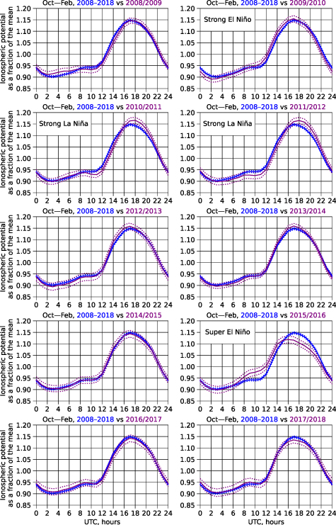
Figure 2. Diurnal variation of the ionospheric potential in the 5 month period around December (October–February) on average (on the basis of the data for 2008–2018; blue solid lines) and in each particular year (purple solid lines). The values of the ionospheric potential are given as fractions of the respective diurnal means. Dotted lines show diurnal variations plus and minus one standard error (for more details on calculating standard errors in this study, see supplementary information). Opposite systematic deviations of the diurnal variation curve from the long-term mean can be identified during strong El Niños (2009/2010, 2015/2016) and La Niñas (2010/2011, 2011/2012).
Download figure:
Standard image High-resolution image4. Temporal variations of ENSO and the GEC
Now we shall quantify the observations made above. To identify different phases of ENSO, it is common to use various indices based on SST anomalies in different regions of the Pacific Ocean. Here we also use this approach, focusing our research on the so-called Niño 3.4 region, defined as the area bounded by 5∘ N and 5∘ S in latitude and by 120∘ W and 170∘ W in longitude; the value of the SST averaged over this region is referred to as the Niño 3.4 SST (see supplementary information for technical details of its computation).
4.1. Definition of anomalies in the Niño 3.4 SST and in the relative IP
SST anomalies in the context of ENSO are usually computed relative to long-term averages taken over several decades. Considering that in this study we want to compare SST anomalies with the corresponding irregularities in the GEC behaviour, here we calculate all anomalies relative to the 11-year averages over the 2008–2018 period, for which we have the data on the atmospheric dynamics and the simulated diurnal variation of the IP. Here are precise definitions that we use in this study.
Let T be the diurnal mean of the Niño 3.4 SST; T can be regarded as a function of the date. We denote by  the value of T averaged over the 5 month interval around the month m of the year y, and we denote by
  the value of T averaged over the same 5 months of all years available in our data (2008–2018). Now we define the anomaly AT of T as a function of the month m and year y as follows:
the quantity AT measures the deviation of T around the month m of the specific year y from typical values for the same time of year; the averaging over 5 month periods, typical for studies of ENSO, is employed to reduce the impact of various short-term effects and focus on the long-term behaviour of T. For example, if we consider November 2014 (m = 11, y = 2014) then  is the average of T over September 2014–January 2015, while
  is the average of T over all available Septembers, Octobers, Novembers, Decembers and Januaries. The anomaly AT(11, 2014) shows the deviation of the mean T around November 2014 from the values that T typically has around November.
Similarly, let V be the IP; V can be regarded as a function of the date and the UTC hour h. For each h we define  and
and  just as we have defined
  and
and  above. Now we define the anomaly AV of the relative IP as a function of m, y and h in the following way:
where  denotes the 24 h average of f(h) over h (i.e. here we deal with relative diurnal variations of V). The quantity AV[h] characterizes the deviation of the value of V at the UTC hour h (relative to the diurnal mean) around the month m of the year y from typical values for the same time of year.
To put it simply, the anomalies defined above measure the deviation of variables from their long-term averages for the same time of year, with a 5 month moving average applied to each parameter.
4.2. Comparison of anomalies in the Niño 3.4 SST and in the relative IP
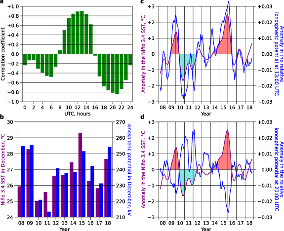
Having defined anomalies in the Niño 3.4 SST and in the relative IP, we now want to compare them in order to identify the effect of ENSO on the diurnal variation of the GEC. The values of the sample correlation coefficient between anomalies in the Niño 3.4 SST and in the hourly values of the relative IP are presented in figure 3(a). These correlations have been estimated on the basis of the 128 months for which the surrounding 5 month periods, used for averaging in the definition of anomalies, lie completely in 2008–2018 (i.e. March 2008, April 2008, May 2008 and so on up to October 2018). Analysis shows that the correlation between the Niño 3.4 SST and relative IP is statistically significant at the 1% level for all hours of the day except 1:00, 2:00, 8:00 and 16:00 UTC (for more details, see supplementary information). We can identify a period of high positive correlation at 9:00–15:00 UTC and a period of high negative correlation at 18:00–23:00 UTC, which generally confirms our observations of the IP behaviour during ENSO events made in section 3.
Figure 3. (a) Sample correlation coefficient between anomalies in the Niño 3.4 SST (AT) and in the hourly values of the relative ionospheric potential (AV[h] for different h's). The correlation is statistically significant at the 1% level for all hours of the day except 1:00, 2:00, 8:00 and 16:00 UTC (for more details, see supplementary information). (b) Average values of the Niño 3.4 SST (purple bars) and the ionospheric potential (blue bars) in December. For clarity the ionospheric potential values are normalized such that their mean over 2008–2018 is equal to 240 kV. (c) Comparison between the anomaly in the Niño 3.4 SST (AT, purple curve) and the anomaly in the relative ionospheric potential at 13:00 UTC (AV[13:00], blue curve). (d) Comparison between the anomaly in the Niño 3.4 SST (AT, purple curve) and the anomaly in the relative ionospheric potential at 21:00 UTC (AV[21:00], blue curve). Areas filled with light red and light blue in panels (c) and (d) correspond to strong El Niños and strong La Niñas respectively; pronounced anomalies of the Niño 3.4 SST during these events are accompanied by pronounced anomalies in the relative ionospheric potential at 13:00 and 21:00 UTC. Note that a 5 month moving average has been employed in calculation of all anomalies.
Download figure:
Standard image High-resolution image
The correlation coefficient between the Niño 3.4 SST and relative IP has a maximum of 0.90 at 13:00 UTC and a minimum of −0.83 at 21:00 UTC. The long-term variations of the anomalies in the relative IP for these hours are shown in figures 3(c) and (d) by blue lines; the plots are based on 128 values corresponding to the same months as above. Comparing these variations against the variation of the anomaly in the Niño 3.4 SST, shown by purple lines in the same panels, we conclude that pronounced El Niño and La Niña events (those with the anomaly in the SST about or greater than 1 ∘C) are associated with pronounced anomalies in the relative IP around 13:00 UTC and 21:00 UTC. More precisely, during strong El Niños (indicated by areas filled with light red in figures 3(c) and (d)) there are prominent positive anomalies in the relative IP at 13:00 UTC and negative anomalies in the relative IP at 21:00 UTC; by contrast, strong La Niñas (areas filled with light blue) are characterized by pronounced negative anomalies in the relative IP at 13:00 UTC and positive anomalies in the relative IP at 21:00 UTC. In other words, during strong El Niños the relative IP is higher than usual around 13:00 UTC and lower than usual around 21:00 UTC, whereas during strong La Niñas it behaves oppositely; this also agrees with the observations of section 3.
4.3. Comparison of the Niño 3.4 SST and the average IP in December
In this paper we primarily focus on changes in the IP values divided by the corresponding diurnal means. Let us now briefly look at the absolute values of the IP. Figure 3(b) presents the monthly values of the simulated IP in December (when ENSO events are most pronounced) together with the corresponding monthly average SSTs. The two data sets are positively correlated with a correlation coefficient of 0.70, which means that absolute IP values are also influenced by ENSO. However, we observe that the year-to-year variability of the average IP does not clearly reflect strong El Niño and La Niña events (to see this, it suffices to compare the IP values for 2008, 2009, 2015 and 2018 in figure 3(b)); on the other hand, for anomalies in the relative IP, shown in figures 3(c) and 3(d), we have seen a precise correspondence. It is apparent that the absolute IP values are influenced by other factors besides ENSO as well; these issues require further investigation beyond the scope of our present analysis.
It is interesting that Harrison et al (2011), who analysed the results of atmospheric electricity measurements at the Shetland Islands during 1968–1984, arrived at a similar finding for the electric field: a clear positive correlation between the Niño 3.4 SST anomaly and the mean surface electric field in December without exact correspondence of the most pronounced anomalies (see their figure 1(a)). However, they did not consider changes in the relative diurnal variation, on which we focus in this article.
5. Further discussion and further implications
Our results imply that ENSO has a significant effect on the GEC intensity, consistently modifying the shape of the Carnegie curve. Considering that our conclusions are based on the long-term simulation of atmospheric dynamics on the basis of real meteorological data, it is clear that the physical mechanism behind the observed influence is related to the variability of the spatial distribution of global electrified clouds, which maintain the GEC, with the ENSO cycle. According to our simulations, the most pronounced changes in the global distribution of convection (and, by inference, in the distribution of electrified clouds) during El Niños and La Niñas occur over the Pacific Ocean, Maritime Continent and South America; however, here we shall not go into a detailed investigation of this matter, leaving it for later studies.
It is important to note that, considering that different GEC parameters are related to each other and have nearly the same diurnal variations, perturbations corresponding to ENSO events should be detectable not only in the behaviour of the IP, which is rather difficult to measure on a regular basis, but also in the dynamics of the surface fair-weather electric field or air—Earth current. Thus it should be possible to find the effect of ENSO in the results of atmospheric electric field measurements. Note, however, that surface atmospheric electricity measurements are influenced by highly variable local factors and usually require averaging over a large number of days to eliminate their influence. Therefore, it is likely that the rather subtle effect predicted by our modelling (see figure 2) will be difficult to find in the surface electric field data for each individual El Niño or La Niña event. At the same time our simulations yield an important conclusion that anomalies in electric field values relative to the diurnal mean are expected to represent the ENSO cycle better than daily mean values themselves, which do not clearly reflect strong El Niños and La Niñas (compare figure 3(b) with figures 3(c) and (d)); this should be especially important for analysing the results of measurements.
6. Conclusions
Modelling the GEC variability during 2008–2018 allowed us to identify a new statistically significant relationship between the GEC and ENSO. According to our simulations, strong El Niño and La Niña events influence the global distribution of electrified clouds over the Earth's surface and thus consistently affect the shape of the diurnal variation of the GEC. For example, at the peak of the super El Niño event of 2015–2016 the relative IP was clearly above the long-term mean at 7:00–14:00 UTC and below it at 16:00–23:00 UTC; the effect of the 2009–2010 El Niño on the GEC was somewhat similar, whereas La Niñas in 2010–2011 and 2011–2012 resulted in the opposite behaviour (precise hours when the changes in the relative IP are most pronounced are slightly different depending on the event; future analysis of the results of long-term atmospheric electricity measurements should make this inference more concrete and eliminate simulation uncertainties). Further analysis of simulation results shows that anomalies in the Niño 3.4 SST and in the relative IP exhibit a strong positive correlation at 9:00–15:00 UTC and a strong negative correlation at 18:00–23:00 UTC. This correspondence is most prominent at 13:00 UTC and 21:00 UTC, and pronounced anomalies in the relative IP around these hours are associated precisely with pronounced El Niño and La Niña events. In particular, this implies that IP values relative to the diurnal mean follow the ENSO cycle in a more distinct way than average IP values, whose behaviour does not clearly reflect strong El Niños and La Niñas. During strong El Niños the relative IP is larger than usual around 13:00 UTC and smaller than usual around 21:00 UTC, whereas during strong La Niñas it behaves oppositely.
Acknowledgment
This work was supported by a grant from the Government of the Russian Federation (Contract No. 075-15-2019-1892).
Data availability statement
The WRF-ARW model can be downloaded from www2.mmm.ucar.edu/wrf/users/downloads.html. The NCEP FNL Operational Model Global Tropospheric Analyses data set, used for the model initialization, is available at https://rda.ucar.edu/datasets/ds083.2. Source codes and scripts used to analyse the results of simulation and plot the images are available at https://bitbucket.org/nilyin/enso-gec-2020.
Author contributions
N V I performed WRF runs and ionospheric potential computation. N N S and N V I analysed the results of calculations and prepared the figures. N N S, N V I, E A M and C G P contributed to the interpretation of the results and writing of the paper.