

Abstract
Winter precipitation estimations and spatially sparse snow observations are key challenges when predicting snowmelt-driven floods. An improvement in streamflow prediction is achieved in a snowmelt-dominant basin, i.e. the Red River Basin (RRB), by adjusting the amounts of snowfall through satellite-borne passive microwave observations of snow water equivalent (SWE). A snowfall forcing dataset is scaled to minimize the difference between simulated and observed SWE over the RRB. Advanced microwave scanning radiometer-E (AMSR-E) SWE products serve as the observed SWE to obtain the solution to the linear equation between the AMSR-E and the baseline (no snowfall-forcing adjustment) SWE to yield a multiplication factor (Mfactor). In the headwaters of the RRB in the United States, a Nash–Sutcliffe efficiency (NSE) of 0.74 is obtained against observed streamflow, with Mfactor-adjusted streamflow during the snowmelt seasons (January to April). The baseline streamflow simulation without Mfactor exhibits an NSE of 0.38 owing to an underestimated SWE.
Export citation and abstract BibTeX RIS

Original content from this work may be used under the terms of the Creative Commons Attribution 4.0 license. Any further distribution of this work must maintain attribution to the author(s) and the title of the work, journal citation and DOI.
1. Introduction
Cold region hydrological processes have garnered increasing attention because of climate change and its hydrological effects on communities where snow and ice are essential to the water supply [1]. Estimation of the amount of snowmelt runoff remains challenging despite long-term concerns regarding the applications of water resources, which are associated with snow hydrology [2–5]. Cold region hydrological processes have different characteristics that are affected not only by rainfall, but also by the release of snowmelt, which depends on the distribution of the snow water equivalent (SWE) and the timing of melts in the basin. In climatology, in addition to the finer-scale hydrological cycle, snow is regarded as a sensitive element for the evaluation of climate variations at both local and global scales [6].
Winter precipitation corrections for mountainous areas have been attempted by many researchers for hydrologic modeling applications [7, 8]. Adams and Lettenmaier [9] adjusted the bias of global winter precipitation, but the source of adjustments was from point-based meteorological observations. Andreadis and Lettenmaier [10] assimilated the SWE using a remote sensing dataset, including passive microwave observations; however, streamflow was not simulated as a criterion for performance improvement. Shi et al [11] evaluated cold region hydrological processes in the Northern Hemisphere using bias-corrected winter precipitation to demonstrate recent changes induced by climate change in the cryosphere to evaluate the degree to which streamflow prediction is improved using the adjusted winter precipitation in subarctic watersheds. Despite the importance of snow, exact mass measurements and spatially varying snowfall monitoring are unreliable when using traditional or sophisticated observational technologies, including in-situ precipitation gauges, and ground-based precipitation radars [12]. Furthermore, measurement errors associated with a precipitation gauge range from 20% to 50% as compared with the actual snowfall; this is typically referred to as the 'snow undercatch' problem [13, 14]. Approximately half of all snowflakes at high wind sites tend to be recorded using traditional precipitation gauges owing to aerodynamic flows around the gauge [15]. This suggests that a multiplication factor of approximately 2 is necessitated to accommodate the actual amount of snowfall to a land surface at open and windy sites, such as the Northern Great Plains. If a device for precipitation measurement is affected by snow undercatch, and a weather forcing dataset is generated from these point precipitation observations, then a scaling factor to correct the winter precipitation must be applied. Additionally, the factor must be constant across a watershed, regardless of temporal variations. Owing to the heterogeneous distribution of terrestrial snow on complicated topographies, it is challenging to determine the scaling factor in a watershed.
Few modern snow hydrologic applications using remote sensing have been implemented in the Northern Great Plains [16, 17], as compared with the numerous snow studies in the western United States. In the Northern Great Plains, snow is the most detrimental source of flooding during spring snowmelt. Snowmelt-driven floods directly affect the population along the rivers in the Northern Great Plains [18, 19] because of the flat topography and poorly draining soil. These factors decrease the flow velocity of surface waters derived from the snowmelt once it begins [20]. To demonstrate an improvement in streamflow prediction by adjusting winter precipitation, a representative and well-observed watershed, the Red River Basin (RRB) in the Northern Great Plains, was investigated. The headwaters of the RRB were selected to apply the proposed multiplication factor (Mfactor) method to the underestimated winter precipitation to demonstrate the improvement in streamflow prediction.
Streamflow simulation driven by snowmelt involves various nonlinear processes such as selection of snow schemes, infiltration characteristics, and routing schemes after the land model is used. However, this study focused on the effect of snowmelt on streamflow generation in a snowmelt-dominant watershed instead of other hydrological processes. The hydrologic model was used twice, i.e. (a) with a baseline hydrologic simulation with non-adjusted winter precipitation; and (b) with an adjusted winter precipitation hydrologic simulation scaled by Mfactor. The scaling factor of the winter precipitation was derived from the solution for linear equations between the advanced microwave scanning radiometer-E (AMSR-E) SWE and the baseline SWE. We independently determined the amount of SWE at each grid cell using the AMSR-E SWE. This was achieved by employing an AMSR-E passive microwave radiometer from the National Aeronautics and Space Administration Aqua satellite for years 2002–2011. Satellite passive microwave products for the SWE are spatially distributed and temporally continuous. Hence, they are appropriate for determining the average amount of SWE over the domain when the SWE is dry and does not exceed 150 mm. The two cases of simulated streamflow (baseline and Mfactor adjusted) were calibrated against the observed streamflow from stream gauge data available from the U.S. Geological Survey (USGS). The hydrologic calibration/validation and streamflow analyses were constrained to the snow-melting period from January to April, not for an entire year. The aim of this study was to determine the scaling factor for winter precipitation in a watershed in the Northern Great Plains for a specified period and then apply it to the prediction of streamflow over a longer period using a hydrologic model to demonstrate an improvement in streamflow performance during the melt season.
2. Methods and materials
This section provides details regarding the methods for scaling winter precipitation using the solution for linear equations between the AMSR-E SWE and the baseline hydrologic simulation. First, a description of the application watershed is presented, followed by the specifications of the hydrologic model and a method for adjusting winter precipitation.
2.1. RRB in the in the Northern Great Plains
The RRB flows through two U.S. states and one Canadian province, starting at the border between North Dakota and Minnesota, and ending in Manitoba, Canada. The catchment of this north-flowing river occupies 287 500 km2, and springtime ice congestions in the north result in considerable flooding because of the backwater effect of these frozen water bodies [21]. In recent decades, the RRB has experienced regular annual flooding incidents, causing national-level concern [22]. The floods from January to April are primarily driven by fast snowmelt. Significant community efforts have been expended with support from state and federal governments [23] to establish flood prediction and monitoring capabilities for residents throughout the main stem of the RRB. It is critical to establish a monitoring system for spatially distributed SWEs. Satellite passive microwave observations, with revisits twice per day, can be used to determine the daily status of the SWE throughout the basin, thereby allowing observations of the peak amount of SWE.
Figure 1 (left) depicts the location and extent of the RRB headwaters, to which this study was applied, which has an area of 13 476 km2. The outlet of the RRB headwaters is located in Fargo, ND and was gauged using the USGS streamflow gauge ID 05054000. The enlarged view of the watershed in figure 1 (center) provides a topographic representation of the RRB; the elevation difference over 130 km of the river was 200 m, with an average slope of only 0.08°. The large area of the basin and the rapid increase in air temperature during the spring season resulted in abrupt flooding in the local municipalities, particularly along river banks in the Fargo metropolitan areas. An abrupt increase in the air temperature, coupled with the flat topography, caused a free water body to form from the meltwater, and small melt ponds enlarged abruptly owing to the poor drainage of the Northern Great Plains. The average maximum winter precipitation, from December to March, is approximately 100 mm SWE, which is sufficient to create a large snow mass. During wet winters, the peak SWE in the large basin can reach up to 200 mm, which is disastrous to many communities when any abrupt melting occurs in the spring. For a general depiction of the climatology of this region, figure S1 (available online at stacks.iop.org/ERL/16/044055/mmedia) demonstrates the monthly snowfall, rainfall, and air temperature averaged from 1995 to 2013 in the headwaters of the RRB.

Figure 1. Left: location of headwaters of RRB (center): headwaters and subwatersheds of RRB as well as locations of USGS streamflow gauges, and (right): two sets of hydrologic simulations with and without Mfactor for evaluating streamflow predictability. Arrows show sequential steps of Mfactor and the variable infiltration capacity (VIC) applications for streamflow evaluations.
Download figure:
Standard image High-resolution image2.2. VIC-ROUT model setup
In this study, a semi-distributed macroscale hydrological model known as the VIC model (version 4.0.6) was used [24] in addition to a routing scheme, VIC-ROUT. The VIC model has been widely applied to assess hydrological responses to weather and climate over numerous river basins globally [for example, 25, 26]. The VIC model was used in this study for streamflow calibrations, with emphasis on the snowmelt runoff in the headwaters of the RRB in the Northern Great Plains. Detailed descriptions of the snow scheme are included in pages 6–9 of the supplementary data. Precipitation and temperature observations were provided by weather stations, and the synergraphic mapping system algorithm [27] was employed to generate gridded temperatures spatially interpolated from the point observations [26, 28]. Specifically, the precipitation data were obtained from NOAA cooperative observer (COOP) stations using standard precipitation gauges. Wind speeds were obtained from a reanalysis dataset from the National Centers for Environmental Prediction–National Center for Atmospheric Research [29]. Point measurements were linearly interpolated from approximately 1.9° to 1/8° resolution, which is similar to the grid resolution used in the AMSR-E SWE retrieval.
With the baseflow and runoff from the VIC considering snowmelt with three soil layers, classic streamflow calibration was performed by minimizing the cost function between the observed and simulated streamflows at the outlets of a watershed [30, 31]. Calibrated soil parameters were applied to the validation period to evaluate the accuracy of streamflow prediction. It is beyond the scope of this study to identify the optimal soil parameters to accurately represent the overall peak of the streamflow associated with rainfall and snowmelt.
2.3. Winter precipitation adjustment using AMSR-E SWE
The amount of winter precipitation in the model was adjusted with a factor to match with the amount of SWE based on the U.S. AMSR-E SWE product (25 km), compared with the 12.5 km grid cell of the VIC model. A Mfactor of winter precipitation was used to scale the winter precipitation in relation to the observed AMSR-E SWE. Despite the well-known microwave saturation that occurs when the SWE exceeds 150 mm [32–34], the AMSR-E SWE offers several advantages, including long temporal coverage (2002–2011), near-daily observations, and global spatial coverage [35]. The National Snow and Ice Data Center (NSIDC) archives the microwave brightness temperature (Tb). The SWE products from the AMSR-E Tb datasets were processed based on a spectral difference between the 18.7 GHz Tb (least affected by snow) and the 36.5 GHz Tb (most affected by snow [36],). The period from 2002 to 2011 was used to encompass the global domain with a 25 km grid using the equal area scalable earth grid (EASE-Grid) format from the NSIDC (later updated to EASE-Grid 2.0 [37]). A spatially averaged ratio was obtained using a solution for linear equations between the AMSR-E based observed and the baseline simulated SWE in all grid cells throughout the hydrologic years from 2003 to 2011. The Mfactor was calculated using the following equation:

where SWEAMSR-E is the AMSR-E-retrieved daily SWE (mm), and SWEVIC-baseline is the VIC-simulated daily SWE (mm) without Mfactor adjustment. Mfactor is determined by solving a system of linear equations with the assumption that both time series are row vectors of the same size from hydrological years 2003–2011. It is noted that Mfactor is determined by considering the entire hydrologic year, and it is specific to the basin where the Mfactor method is applied. A classical  solution for the linear equations is represented by the Moore–Penrose pseudoinverse [38, 39] of SWEVIC-baseline (A) owing to the non-invertibility of its row vector. Subsequently,
  is multiplied by SWEAMSR-E (B), which is the left term of the right-hand side in equation (2), to obtain Mfactor on the left-hand side. Physically, this system solution of the linear equations only accounts for days when snowfall appears for both the SWEVIC-baseline and SWEAMSR-E cases. Specifically, the Mfactor for the headwaters of the RRB was 2.53. It is noteworthy that 2.53 was derived by applying equation (1) to the headwaters of RRB; however, its values typically vary from 2 to 3 when applied to the other subwatersheds of the RRB.
Furthermore, the winter precipitation was multiplied by Mfactor during the hydrologic modeling period, i.e. 1995–2013, by assuming that the AMSR-E SWE sufficiently captured the underestimated baseline SWE even outside of the period where Mfactor was calculated. The National Oceanic and Atmospheric Administration National Climatic Data Center and COOP (hereinafter NOAA COOP) weather stations and SNODAS [40] snow assimilation data can be used to replace the AMSR-E SWE; however, it is only applicable to well-observed watersheds such as the RRB, where the number of observations is abundant. However, snow undercatch problems persist in NOAA COOP stations.
Figure 2 displays three basin-averaged SWE estimates: the baseline VIC simulation, the Mfactor-adjusted VIC simulation, and the AMSR-E SWE observations. The spatially averaged ratio from equation (1) during the Mfactor calculation period, i.e. 2003–2011, was used as the scaling factor for the winter precipitation at all 70 grid cells in the RRB headwater region and was applied to the longer hydrologic modeling period, i.e. 1995–2013, to demonstrate the validity of Mfactor outside the Mfactor calculation period. A Mfactor-adjusted hydrologic simulation was performed to demonstrate the improved predictability of snowmelt-driven floods. A schematic illustration is shown in a block diagram in the right panel of figure 1 to show the Mfactor calculation period from 2003 to 2011. The hydrologic simulation from 1995 to 2013 was independent of Mfactor calculation to calibrate the soil parameters and had a wide temporal range. A hydrologic calibration scheme was applied to two cases: a baseline VIC simulation without Mfactor and a VIC simulation with Mfactor. Streamflow calibrations were conducted by fitting to the observed streamflow for both cases, from January to April, to adjust the soil parameters. The two applications illustrate the degree to which Mfactor affects the SWE, followed by the extent to which the winter precipitation adjustment aided by passive microwave observations improved the streamflow prediction during the subsequent months of melt-runoff.

Figure 2. SWE intercomparison among VIC baseline, Mfactor-adjusted, and AMSR-E-retrieved SWEs. Mfactor calculation period (2003–2011 hydrological years) and hydrologic simulation period (1995–2013) shown below x-axis.
Download figure:
Standard image High-resolution image3. Results and discussion
First, monthly averaged streamflows for both the calibration and validation periods are presented using the baseline and Mfactor-based streamflow simulations as well as Nash–Sutcliffe efficiency (NSE) values [41]. Additional streamflow results are based on three events selected from historic floods in Fargo, ND. Monthly streamflow analyses with embedded plots of the monthly SWE demonstrate the extent to which SWE affects spring snowmelt, and the degree of improvement in streamflow prediction based on the AMSR-E aided SWE adjustment during extreme floods.
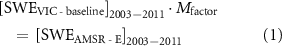
3.1. Calibration and validation: baseline simulation vs. Mfactor-adjusted simulation of RRB headwaters
The calibration and validation periods were 1995–2007 and 2008–2013, respectively, and Mfactor was applied to both periods. It is noteworthy that the calibration was only applied from January to April when spring snowmelt was the dominant factor determining peak streamflow. The simulated streamflow using the Mfactor SWE more accurately replicated the observed streamflow during both the calibration and validation periods, compared with the streamflow from the baseline SWE. The Mfactor-driven streamflow during the calibration period achieved an NSE of 0.74 for the snowmelt-runoff season. The VIC baseline streamflow was underestimated against the observed streamflow, even with the annually averaged streamflow, as reflected by the low NSE of 0.38. Additionally, the validation period showed the underestimation of the baseline streamflow simulation, but the degree of underestimation was lower than that for the calibration period. The NSE values were 0.48 and 0.11 for the Mfactor and baseline streamflow simulations, respectively. The relatively low NSE during the validation period was attributed to the short validation period of only 6 years, and differences from the streamflow peak were associated with the timing of snowmelt. Furthermore, streamflow calibration was not applied to the periods October–December and May–September when snowmelt was not the main contributor of floods.
3.2. Floods in 1997, 2010, and 2011
It is noteworthy that hydrologic calibration was only applied from January to April in this study. Figure 3 shows the monthly averaged streamflow performance during the hydrologic simulation period, and these results suggest that all the hydrological years contributed to a stable improvement in the streamflow predictions corresponding to January to April. However, as shown by the event-based simulations of streamflow in figure 4, the improvement in the flood prediction was apparent only during the snowmelt season within the shaded areas. Figure 4 (top) shows the baseline, Mfactor-driven, and USGS-observed streamflows for the historic 1997 flood in Fargo, ND. The baseline, SWE-adjusted, and USGS-observed streamflows were plotted using the left-hand y-axis. The predicted streamflow was nearly identical to the USGS streamflow in April 1997, with a peak of 500 m3 s−1, which was attributed to the increasingly adjusted SWE shown in the right y-axis, in the reverse direction (also represented in figure S2). The matching of streamflow in the spring of 1997 suggests that the adjusted amount of winter precipitation from the AMSR-E SWE may improve the streamflow prediction of the observed precipitation. This successful identification of the peak streamflow was achieved in 1997 without the availability of AMSR-E SWE. This implies that the Mfactor calculated from 2002 to 2011 is also valid in 1997, thereby allowing an accurate capture of peak streamflow.
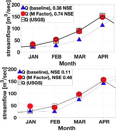
Figure 3. (top) Monthly averaged streamflow from 1995 to 2007 (calibration period); comparison among VIC baseline, Mfactor-driven simulation, and observed streamflows. (bottom) Monthly averaged streamflow from 2008 to 2013 (validation period).
Download figure:
Standard image High-resolution image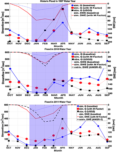
Figure 4. Baseline, Mfactor-driven, and observed streamflows (left axes), and SWE (right axes). Hydrologic years are 1997 (top), 2010 (middle), and 2011 (bottom).
Download figure:
Standard image High-resolution image
In the hydrological years of 2010 and 2011, the AMSR-E SWE was available, and the VIC baseline streamflow continued to underestimate the observed streamflow. The Mfactor-adjusted winter precipitation resulted in an improved prediction of streamflow that was comparable to the USGS peaks for March 2010 and April 2011. The prediction for 2010 indicated better performances than those for 2011; this is attributable to the difference in the timing of the SWE peaks in 2011 between the AMSR-E (in February) and the baseline (in January), as shown at the bottom of figure 4. Interestingly, the baseline VIC streamflow simulation could not capture the low observed streamflow in June and July. This was because the adjusted soil parameters from January to April promoted runoff and baseflow, which are associated with the spring snowmelt, thereby resulting in increased streamflow; however, it was insufficient to reflect the observed peak in streamflow. The SWE-adjusted Mfactor streamflow, however, successfully identified the observed spring peak as well as moderately dry streamflow following snowmelt floods in June and July, which are rainfall-dominated months. In contrast to the baseline, the relatively better performance of Mfactor from May to September was associated with the calibrated soil properties from the Mfactor simulation from January to April, which was applied equally to the other months. The relatively poor performance of the Mfactor streamflow during January and February was caused by a difference between rainfall-runoff and snowmelt-runoff. Snowmelt runoff has a longer lead time than rainfall-runoff, i.e. the released water requires a longer time to arrive at the land surface; therefore, a discrepancy occurs between streamflow predictions in January and February, as well as those in March and April.
4. Conclusions
In this study, the accuracy of streamflow predictions conducted using a baseline simulation method was compared with that obtained from simulated streamflows based on the SWE, which was adjusted by scaling winter precipitation using passive microwave observations. The headwaters of the RRB in the Northern Great Plains were selected because the precipitation gauges exhibit typical snow undercatch, and weather forcing datasets are available from those point measurements. The conclusions of this study are as follows:
- The 'snow undercatch' by standard precipitation gauges was confirmed by the underestimated streamflow in the RRB headwaters in the baseline simulation. This winter precipitation forcing [26, 28] underestimation was resolved by applying Mfactor to adjust the amount of winter precipitation. The Mfactor was calculated as the ratio of the AMSR-E-retrieved SWE to the baseline VIC simulation SWE. The underestimated SWE resulted in an underestimated peak streamflow during snowmelt. The VIC simulation with the adjusted SWE (Mfactor) performed significantly better, with a 0.74 NSE for the snowmelt-dominant watershed, compared with a 0.38 NSE of the baseline simulation.
- SWE values in the Northern Great Plains range from 50 to 100 mm, which is below the sim150 mm saturation limit of the AMSR-E SWE algorithm.
- The 1997 historic flood exhibited a peak flow of 500 m3 s−1 and was successfully captured by the SWE-adjusted VIC-ROUT simulation. It is noteworthy that the 1997 hydrological year is outside the period when Mfactor was calculated. This streamflow prediction implies that the assumption of Mfactor is valid for snow hydrologic processes outside the Mfactor calculation period.
However, some limitations were discovered: The AMSR-E SWE retrieval began saturating at 150 mm and was valid only under dry snow conditions [32–34]. Nonetheless, further studies can be conducted, such as in downstream basins whose outlets are in the Grand Forks, ND, US and Winnipeg, Manitoba, Canada. These areas offer larger watersheds for characterizing the general snowmelt-runoff generation in the Northern Great Plains. It would be valuable to extend the algorithm to snowmelt-driven, environmentally vulnerable, and measurement-limited watersheds where oil sands are being excavated in the far northern prairie of North America [42]. Snowmelt-driven floods are increasingly reported in Central Asia and the Northern Caucasus, where the climate and topographical conditions are similar to those in the Northern Great Plains [43, 44]. In such regions, undertaking environmental observations is challenging, and the source and errors of measurements of winter precipitation forcing are known. This study focused on evaluating the applicability of a satellite-borne passive microwave SWE dataset to improve streamflow estimation by hydrologic modeling in a limited headwater basin. This enabled us to emphasize the importance of SWE observations for streamflow generation in cold-region hydrology.
Acknowledgments
This research was supported by the first author's appointment to the NASA Postdoctoral Program at the Goddard Space Flight Center, and another the NASA grant, 80NSSC18K1136.
Data Availability Statement
AMSR-E Daily SWE is available through Tedesco et al [36] archived at the National Snow and Ice Data Center. Codes for VIC 4.0.6 are available at https://github.com/UW-Hydro/VIC/tree/master/vic/vic_run. USGS streamflow data in Fargo, ND, USA, is from: U.S. Geological Survey, 2016, National Water Information System data available on the World Wide Web (USGS Water Data for the Nation), accessed (11 February 2021), at URL (https://waterdata.usgs.gov/usa/nwis/uv?05054000).
No new data were created or analysed in this study.