

Abstract
Concrete is the most produced manmade material globally. This widespread production results in significant anthropogenic environmental impacts, the awareness of which has spurred advances in material development to lower these burdens. However, proposed changes are often not assessed in the context of the data variability and uncertainty inherent in the environmental impact quantification methods employed. As such, the probability that any suggested strategy will result in a desired effect is not addressed. This work aims to quantitatively examine data variability, an inherent characteristic of elements in supply chains, and data uncertainty, a function of data quality for the system being modeled, in assessments of greenhouse gas (GHG) and air pollutant emissions from concrete production. Data variability is determined through ranges in requisite input values from the literature; data uncertainty is assessed through application of an established pedigree matrix method. Statistical analysis of the emissions from concrete production incorporating sources of variability and uncertainty are examined through Monte Carlo simulations. Concrete mixtures, representing a feasible structural concrete for use in California infrastructure and three alternative mixtures are assessed, as are three GHG emissions mitigation strategies, namely, a change in thermal energy fuel mix, a change in electricity grid, and use of carbon capture and storage. The distributions of emissions derived through statistical analyses are used to examine the probability of efficacy of these strategies, as well as potential co-benefits on air emissions. Results show each constituent change and each mitigation strategy considered would lead to a reduction in GHG emissions if only mean values are compared; however, the probability of these reductions varies. These findings suggest mitigation efforts may not be as definitive as current assessments suggest. Results indicate the importance of using statistical methods to target desirable mitigation efforts in the environmental impacts from concrete production.
Export citation and abstract BibTeX RIS

Original content from this work may be used under the terms of the Creative Commons Attribution 4.0 license. Any further distribution of this work must maintain attribution to the author(s) and the title of the work, journal citation and DOI.
Abbreviations
| CO | carbon monoxide |
| FA | Class F fly ash |
| NOX | nitrogen oxides |
| PC | Portland cement |
| Pb | lead |
| PM2.5 | particulate matter of under 2.5 µms |
| PM10 | particulate matter of under 10 µms |
| SCM | supplementary cementitious material |
| SOX | sulfur oxides |
| VOCs | volatile organic compounds. |
1. Introduction
The environmental impacts from the widespread production of concrete have sparked concerted efforts to find appropriate mitigation strategies. Concrete, which is composed of several materials including cement, aggregates, water, and when applicable, admixtures and/or reinforcing fibers, is currently the second most used material by humans after water [1]. Current production of cement and its composites, such as concrete, result in approximately 8%–9% of global anthropogenic greenhouse gas (GHG) emissions [2], 2%–3% of energy use worldwide [1], and 1%-2% of global water withdrawal [3]. The production of concrete generates other key environmental impacts, such as emissions of particulate matter, sulfur dioxide, nitrogen oxides, and carbon monoxide [4–6].
Increased awareness of these notable environmental impacts has spurred many advances in material development. Through use of environmental impact assessment methods, such as life cycle assessment, academia and industry have been pushing to better understand and mitigate impacts from concrete production [7]. Work on development of life cycle inventories and life cycle assessments for concrete have included fundamental assessments of emissions from the production of concrete and its constituents (e.g. [4, 8–11]), comparisons of specific concrete mixtures and associated compressive strength or other material properties (e.g. [12–14]), and the potential of impact reduction through mitigation strategies (e.g. [2, 15–17]). Work has extended to international organizations, such as the United Nations Environment program [18] and the International Energy Agency [19]. Many of these studies examine the influence of using supplementary cementitious materials (SCMs) as partial replacement for cement production, which has high GHG emissions relative to many SCMs [20]. While quantification methods for the impacts of industrial byproducts vary, particularly with regard to allocation of impacts from the primary processes [21], in this work, a method proposed by the United States (U.S.) Environmental Protection Agency (EPA) is applied in which no energy is allocated to the collection of byproduct SCMs [22].
Environmental impact modeling is central to the assessment of environmental burdens of both alternating concrete constituents and alternating manufacturing methods. Yet data uncertainty, a function of data quality for the system being modeled, and data variability, an intrinsic characteristic of the supply chains, are inherent to life cycle environmental impact modeling [23]. These include random error and statistical variation, systemic error and subjective judgment, variability in reported inputs or outputs, and approximation [24]. These sources of variability and uncertainty in environmental impact assessment methods are readily acknowledged [25]; however, they are rarely considered in evaluating mitigation strategies hampering competent decision-making [26]. Recent work has investigated uncertainty in environmental impact assessment along with uncertainty in infrastructure material performance. For example, Lepech et al [27] explored a probabilistic design framework incorporating uncertainty in concrete repairs and rehabilitation along with uncertainty in associated environmental impacts to better engineer sustainable infrastructure systems. Gregory et al [28] proposed a comparative life cycle assessment method that incorporated uncertainty and applied their proposed methodology to a case study of two pavement application scenarios. Chhabra et al [29] explored the extension of performance-based earthquake engineering methods, focusing on steel structures, to incorporate life cycle environmental impacts, while addressing the likelihood that environmental impacts would accrue at different phases. Su et al [30] examined the effects of data uncertainty on the comparisons of environmental impacts associated with insulation materials. Yet, to the author's knowledge, statistical methods for assessing potential efficacy of mitigation strategies for the ubiquitous material concrete remain unexplored. This limitation impedes the ability to select among and implement mitigation strategies that will contribute to emissions goals in a meaningful way.
In deterministic environmental impact assessments of concrete, several indicators have suggested the need for incorporating data uncertainty and variability into comparisons. As noted previously, GHGs and certain air pollutant emissions have been discussed as key impacts that need to be mitigated in the production of cement [6]. Notable levels of variation in GHG and air pollutant emissions have been reported for cement production [31]. Driven from a variety of factors, past studies have noted variability in CO2 and air pollutant emissions from cement production both between plants and over time [32, 33]. GHG emissions and air pollutant emissions from the production of concrete and other building materials have been shown to be strongly a function of the energy and raw material resources used [14, 30, 31]. Energy resources are known to contribute to variability in emissions (e.g. [23, 34]); raw material derived resources have variability often associated with processing conditions, pollution control systems, and chemical composition [31, 35]. As noted previously, beyond this variability, life cycle environmental impact assessment methods are prone to sources of data uncertainty [36]. Based on these factors, this work focuses on raw-material derived and energy-derived (including transportation fuels) contributions to variability and uncertainty in emissions of GHGs and air pollutants in concrete production.
This work aims to formally quantify this variability and uncertainty to understand the probability that mitigation strategies will result in lower GHG and air pollutant emissions from the production of concrete. The production of concrete is studied in California. California has more stringent climate change mitigation policies than the rest of the U.S. [37] and is capable of altering mitigation policy [38]. Due to strong record keeping in the state on energy resources and equipment efficiency in cement manufacture (e.g. [39]), there are fewer sources of uncertainty than data from other areas, representing a current best case scenario, attainable in the near term by other geo-political units. While this one region was selected for analysis, the methods can be extended to other regions.
2. Materials and methods
2.1. Materials
Four concrete mixtures are examined in this work to understand the role of cementitious content on the factors that drive uncertainty in environmental assessments of concrete as well as the potential for alterations in mixture proportions to reduce GHG emissions, while maintaining the same compressive strength. The primary mixture discussed, and used as a baseline for comparisons, was based on the 2018 California Department of Transportation (Caltrans) structural concrete specifications at the high-boundary of cementitious content for a concrete mixture that reaches 25 MPa at 28 days (referred to herein as CA–HC). The influence of changing cementitious content and three procedure changes (discussed hereon as mitigations)- fuel changes, grid changes, and carbon capture (see section 2.2.4) - are examined relative to this CA–HC mixture. The first alternative mixture (CA–LC) uses the low-boundary of cementitious content specified by Caltrans for a concrete mixture that reaches 25 MPa at 28 days. For the CA–HC and CA–LC mixtures, the cementitious contents are 475 and 400 kg m−3, respectively [40]. For these mixtures, 85% Portland cement (PC) and 15% fly ash (FA) were modeled as the cementitious material. FA is among the most common SCMs used; typical usage of FA as a partial replacement for PC by Caltrans is reported in the range of between 15% and 25% [41]. The water content was determined using the factors for Abram's law reported by Fan and Miller [42] for 15% FA mixtures, based on fitting to experimental data from Oner et al [43]. These mixtures result in a notably high water-to-cementitious ratio, but this high ratio leads to viable concrete shown by Oner et al [43]. In applications where this ratio would be considered too great, the use of a water reducing admixture may be desirable. Aggregate content was approximated based on remaining mass of concrete and the ratio between coarse and fine aggregates from Oner et al [43]. Two additional mixtures capable of achieving the same strength at 28 days were examined with lower cementitious content since prescriptive binder contents can often lead to over design. These each used 300 kg m−3 of cementitious material, which was selected as this content has been validated to achieve desired strength properties by Oner et al [43]. Two FA levels were considered with this lower cementitious content: 15% and 30% replacement of PC. The mixture proportions are presented in table 1 and exhibit the role of prescriptive engineering in selection of binder content as well as the role of higher levels of SCM use. The contributions of these concrete constituents to raw-material derived air emissions are addressed in the subsequent section. For this work, the mass of constituents were modeled as not having variability; although, small levels of constituent variability are typically acceptable within certain constraints [40, 44]. While variability of constituent masses was outside the scope of this work, uncertainty in masses specified was included in this study, as discussed in the Methods.
Table 1. Concrete mixtures examined in this work.
| Name | Definition | Constituents (kg m−3) | ||||
|---|---|---|---|---|---|---|
| Portland cement a | FA | Water | Fine aggregate | Coarse aggregate | ||
| CA–HC | Based on Caltrans specifications for at the high end of specified cementitious content | 403 | 71 | 448 | 932 | 405 |
| CA–LC | Based on Caltrans specifications for at the low end of specified cementitious content | 340 | 60 | 378 | 1032 | 449 |
| 300C–15FA | Contains 300 kg of cementitious content with 15% fly ash | 255 | 45 | 283 | 1169 | 508 |
| 300C–30FA | Contains 300 kg of cementitious content with 30% fly ash | 210 | 90 | 266 | 1180 | 513 |
2.2. Methods
2.2.1. Statistical modeling of concrete production emissions models
To assess the role of uncertainty and variability in evaluating the probability of mitigation strategies resulting in reduced environmental impacts from concrete production, this work examines GHG emissions based on carbon dioxide (CO2), methane (CH4), and nitrous oxide (N2O). The three GHG emissions were converted to CO2-eq emissions based on the Intergovernmental Panel on Climate Change 100 year time horizon global warming potentials [45]. This work also examines emissions of several air pollutant emissions: nitrogen oxides (NOX ), sulfur oxides (SOX ), volatile organic compounds (VOCs), carbon monoxide (CO), lead (Pb), and particulate matter of under 10 µms (PM10) and under 2.5 µms (PM2.5).
For the purposes of this work, emissions have been broken into two primary source categories to inform model development: raw-material derived emissions (i.e. emissions resulting from materials themselves) and energy-derived emissions (i.e. emissions resulting from energy resources, including transportation fuels). Distributions of data variability for raw-material or energy-derived emissions associated with each constituent and processes assessed were determined from the literature. If distributions were not available from the literature, then the following distribution types were applied: a deterministic value if only one data point was available; a uniform distribution if two data points were available; a triangular distribution if three data points were available; and a lognormal distribution if four or more data points were available. Additionally, models to capture uncertainty in data were applied as described in section 2.2.3. Variability and uncertainty distributions were propagated through the inventory flows through Monte Carlo simulations (n = 100 000) for production of one cubic meter of concrete for each of the concrete mixtures considered.
2.2.2. Environmental impacts of concrete production
To determine GHG emissions and air pollutant emissions, which are known to have both data variability and uncertainty in assessments of environmental impacts of concrete, process-based environmental impact assessments were conducted. These assessments considered impacts associated from raw material acquisition through concrete production, assuming production in the year 2018; they did not include consideration for construction, service life, or end of life. A simplified process-flow diagram of the scope of this work is presented in figure 1.

Figure 1. Process flow diagram of concrete production. This flow diagram represents common material and energy flows associated with the different phases of manufacturing in concrete production. Processes considered include raw material acquisition and preparation, cement production, use of transportation when appropriate, use of fly ash, and the batching of concrete using these constituents.
Download figure:
Standard image High-resolution imageEmissions from the production of cement are largely affected by location of production. In this work, the PC modeled refers to cement composed of approximately 95% clinker and 5% gypsum by mass (reflective of a CEM I cement, as was used in the experimental data from Oner et al [43] used to model the concrete mixture proportions). Because California produces enough PC to meet its demands [46], it was assumed that PC was produced in-state. In the production of PC, raw-material derived CO2 emissions were approximated as 0.51 kg CO2 emissions per kg of clinker, assuming complete calcination of limestone (CaCO3) to lime (CaO) for a 65% lime-based clinker. Remaining raw-material derived emissions from clinker production were based on data from the U.S. Geological Survey, the Cement Sustainability Initiative's Getting the Numbers Right (GNR) initiative, and the EPA [47–49]. These raw material derived air emissions were calculated as the total emissions reported minus emissions associated with fuel combustion based on U.S. average production (data for raw material derived emissions are reported in the supplementary information (SI) table S.5 (available online at stacks.iop.org/ERL/16/054053/mmedia)).
Energy-related emissions for the thermal requirements of the cement kilns to produce clinker were modeled as a function of kiln efficiency and fuel used. This work uses an average of kiln types in California, namely ∼15% dry kilns and ∼85% precalciner kilns (based on 2005 data from Marceau et al [50]), and energy efficiency based on data reported by the California Air Resources Board (CARB). This energy efficiency was calculated for state production in 2017 based on reported fuel demands [39], lower heating values reported in the GREET tool [51] for common fuels and by Cooper et al [52] for waste fuels, and divided by clinker production reported by CARB [39]. Based on global data reported by GNR [49], typical efficiency variability within kiln types ranges between ±5%. This variability was captured here with a triangular fit for the range of energy demand for these kiln types. The fuel sources were modeled based on data reported by CARB [39] (reported in the SI, table S.8). Distributions for GHG emissions and air pollutant emissions from combustion of these kiln fuels were based on data from [51, 53–55] (distributions for kiln efficiency and emissions from kiln fuels are reported in the SI, tables S2 and S3, respectively).
Beyond the emissions associated with the kiln fuel combustion, energy-related emissions from electricity use at each phase of production were assessed. These electricity demands were evaluated using the efficiency of fuel conversion and electricity demand for different phases of PC production, based on values by kiln type for the U.S [50]. These values were assessed using the average California electricity grid from 2016 (based on [56]; shown in SI table S.9). Variability distributions for GHG and air pollutant emissions factors, except for Pb emissions, by electricity source were based on data from [34]; electricity by different generation methods were weighted by the U.S. use of each generation method from [34]. Pb emissions factors were determined from [57] (emissions factors presented in SI, table S1). Variability for electricity demand was based on the reported differences in electricity demand for cement production in the U.S. between 1990 and 2016 (data from [49]), which was modeled as a triangular distribution with a range of ±5% from the mean. Since PC was considered to be available locally, cement was modeled as being transported 150 km by truck to the batching site. The emissions associated with vehicle transportation were based on two data sources, namely [58, 59], to capture variability.
In addition to the emissions from the production of cement, emissions associated with aggregate production, FA, and concrete batching were assessed. Electricity demand variability for all constituents was modeled as being the same as for cement, a triangular distribution with a range of ±5% from the mean.
For aggregates, production was assumed to take place in California. The raw-material derived emissions of air pollutants from quarrying and/or crushing were based on data from the EPA [55]. Because there were no data available on raw-material derived PM2.5 emissions, they were assumed to be equivalent to PM10 emissions. Additionally, energy-related emissions associated with aggregate quarrying and/or crushing as well as refinement, where applicable, were modeled based on energy demands from Marceau et al [60]. These energy demands were modeled as requiring electricity, and distributions for emissions were based on emissions factors for electricity, accounting for variability, as discussed above, using the California electricity-mix. Aggregates were considered to be sourced locally and transportation of these materials was modeled as a distance of 75 km transported by truck, with distributions for transportation emissions based on [58, 59].
For FA, energy required for capture was estimated as 0 kWh based on estimates from the EPA [22]. Transportation of FA was considered to be 1000 km by rail, based on the closest coal electricity plants, using emissions data from [58, 59]. As a result, the only variability in emissions was that associated with the transportation-fuels (distributions presented in SI table S5).
For the batching stage of concrete production, the electricity demand was based on a report from the Lawrence Berkeley National Lab [61], with emissions factors for this electricity and their variability as discussed above. Additionally, raw-material derived particulate matter emissions during constituent loading, unloading, and transfer were considered (discussed in the SI, section S.2). Water used in concrete batch was assumed to require negligible energy demand to bring it to the batching site.
In this work, data were available for differences in PM10 and PM2.5 emissions from energy resources and emissions from transportation, though such granularity was not available for certain raw-material derived emissions. In these cases, PM10 and PM2.5 emissions were modeled as equivalent (as noted above and shown in data presented in the SI).
It is noted that both chemical composition of raw materials used in concrete constituents as well as storage and/or processing time can influence air emissions. In the production of cement, the composition of raw materials used can influence the magnitude and types of air emissions from clinker production [35]. For all constituents considered, the amount of material lost as fugitive emissions during transportation, transfer, and loading can also play a role in cumulative emissions [62]. Additionally, depending on constituent storage method used and how long those constituents are in storage, wind erosion of stockpiles can lead to air emissions [63]; and changes in practice over time, like the inclusion of improved air emissions controls, can change reported emissions [31]. In this work, the same raw material resources, storage times, and processes were considered within each constituent type, so such time-dependent effects were considered to be limited. Raw-material derived emissions are as discussed above (data modeled are presented in tables in the SI). The additional effects of these sources of variability were outside the scope of this analysis but should be examined in future work.
For each material and stage of concrete production, raw-material derived and energy-derived emissions were cumulatively assessed based on the production of one cubic meter of concrete for each of the concrete mixtures discussed in section 2.1 by using the following formula:
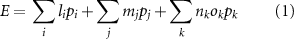
where E is the emissions (calculated separately for each GHG and air pollutant emission), l is the emissions associated with raw-material derived emissions for the production of a constituent, m is the energy-related emissions for each constituent or process, n is the emissions associated with transportation fuel combustion, o is the distance of transportation, and p is the quantity of each constituent. These values are summed over i each type of constituent, j each energy type, i.e. electricity and thermal, associated with each constituent, and k each mode of transportation associated with each constituent.
2.2.3. Uncertainty in inputs
Uncertainty associated with each of the parameters used to examine concrete impacts was assessed with a quantitative pedigree matrix, a common means of assessing several sources of uncertainty in model inputs [64]. In this work, uncertainties were quantified using the method presented by Frischknecht et al [65] and Weidema and Wesnæs [66]. This method facilitates calculation of uncertainty reflecting data quality associated with geographical, temporal, and technological accuracy as well as data reliability and completeness—referred to herein as 'data uncertainty'. Data with lower degrees of reliability, completeness, temporal correlation to this assessment, geographical correlation to this assessment, or technological correlation to the materials and processes being examined were scored with higher factors. These factors were then incorporated into a standard geometric mean to determine data uncertainty for each input. These parameters were then included in the Monte Carlo Simulations to reflect the effects of data uncertainty on anticipated precision of emissions modeled. This method also allows for investigation of the influence of 'basic uncertainty' associated with the uncertainty inherent to types of emissions, that is, uncertainty for each type of emission, regardless of emission source. Using this method, uncertainty associated with emissions from each modeling parameter was quantified. The uncertainty factors applied to each constituent, process, and emission type used, as well as how they were cumulatively assessed for the comparisons drawn are presented in the SI (section S3 and table S7). A list of variable and uncertain parameters considered in this work are shown in table 2.
Table 2. Simplified flows considered in the statistical model derived and list of variable inputs, variable outputs, and uncertainties considered (for a full scope diagram of process flows, see figure 1).
| Inputs | Constituent or process | Emissions to the air | Variable inputs | Variable outputs | Parameters for which data uncertainty was considered |
|---|---|---|---|---|---|
| (a) Electricity demand; (b) kiln efficiency | (a) Raw-material derived particulate matter emissions; (b) thermal energy emissions for each fuel type; (c) electricity emissions for each energy resource; (d) transportation emissions per unit distance traveled | (a) Electricity demand; (b) kiln efficiency; (c) mass of material; (d) raw-material derived emissions; (e) emissions from thermal energy resources; (f) emissions from resources used to provide electricity; (g) transportation distance; (g) transportation emissions; (h) basic uncertainty for each emission type | |||
| (a) Transportation emissions per unit distance traveled | (a) Mass of material; (b) transportation distance; (c) transportation emissions; (d) basic uncertainty for each emission type | ||||
| (a) Electricity demand | (a) Raw-material derived particulate matter emissions; (b) electricity emissions for each energy resource; (c) transportation emissions per unit distance traveled | (a) Electricity demand; (b) mass of material; (c) raw-material derived emissions; (d) emissions from resources used to provide electricity; (e) transportation distance; (f) transportation emissions; (g) basic uncertainty for each emission type | |||
| (a) Electricity demand | (a) Raw-material derived particulate matter emissions; (b) electricity emissions for each energy resource; (c) transportation emissions per unit distance traveled | (a) Electricity demand; (b) mass of material; (c) raw-material derived emissions; (d) emissions from resources used to provide electricity; (e) transportation distance; (f) transportation emissions; (g) basic uncertainty for each emission type | |||
| (a) Electricity demand | (a) Constituent derived particulate matter emissions from batching, transferring, and loading; (b) electricity emissions for each energy resource | (a) Electricity demand; (b) raw-material derived emissions; (c) emissions from resources used to provide electricity; (d) basic uncertainty for each emission type | |||
2.2.4. Mitigation strategies
In addition to assessing impacts of varying concrete constituents, the influence of three mitigation strategies were investigated to quantify the probability that examples of commonly discussed GHG emissions mitigation methods would result in reduced emissions from concrete production. The first mitigation strategy was to use a lower emitting fuel in the cement kilns; specifically, using natural gas as the kiln fuel to replace other fossil fuels. The second strategy was to improve the electricity grid; namely, the grid was assumed to switch to a 100% renewables grid, in which fossil-derived fuels were replaced with wind electricity. The third mitigation strategy modeled was the use of carbon capture and storage (CCS) via amine scrubbing. For this method, an energy demand of 2 GJ t−1 CO2, modeled with the thermal energy mix for the cement kilns, and potential carbon-capture of 90% was modeled, based on [67].
The influence of varying concrete constituents and the three mitigation strategies was assessed relative to the CA–HC mixture using two methods. The first of these was a change in the arithmetic mean between the baseline distribution and the distribution of the emissions associated with concrete containing alternative constituents or with an implemented mitigation strategy. The second comparison was of the probability of reduced GHG emissions or air pollutant emissions, which was calculated by determining the frequency with which reduced environmental impacts were found for each of the simulation runs. Cumulative distribution functions were fit to the differences calculated from these runs, and the probability of reduction was defined as a function of the integral of the cumulative distribution function below 0, as shown in equation (2).
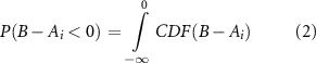
where B is the baseline mixture and Ai is the alternative mixture, for each potential change to constituents or use of mitigations strategies, i.
3. Results
3.1. GHG emission distributions for different concrete mixtures
By incorporating data variability and uncertainty, distributions of anticipated emissions from the production of concrete were assessed. In figure 2, the distributions of the highest cementitious content mixture (CA–HC), which is used in this work as a baseline, and of the lower cementitious content, but same FA level, 300C–FA15 mixture are shown. For these mixtures, the production of PC is the main driver in GHG emissions; the mean contribution of PC to GHG emissions ranged from 89% to 95%, which is within range to published values of emissions for concrete mixtures with similar PC content [13]. Because cement production is the largest contributor to the GHG emissions of the mixtures, the uncertainty associated with this constituent is also the main driver in the distribution of GHG emissions. This finding is noteworthy as the distribution for GHG emissions per kg of PC produced, accounting for data variability and uncertainty, is tighter than the distributions for the other constituents used. However, the high contribution to concrete GHG emissions from this one constituent results in it being a dominating factor for the distribution of GHG emissions for concrete. As a result, the CA–HC mixture has a broader distribution than the lower cementitious content 300C–FA15 mixture. Specifically, the range between the 25% and the 75% quantiles of GHG emissions for the CA–HC mixture is 240–466 kg CO2-eq m−1, but for the 300C–FA15 mixture, the range is 2/3rds that amount. The lowering of PC content could reduce both mean impacts, as has been shown by many studies [68], as well as lower the distribution in impacts; however, such shifts would not be expected across all emissions categories.

Figure 2. Histograms of greenhouse gas emissions for the production of one cubic meter of concrete. This figure represents distributions of GHG emissions for the production of the high cementitious content mixture based on Caltrans specifications (CA–HC) and the mixture containing 300 kg of cementitious material. Mixtures presented contain 15% fly ash replacement of the Portland cement.
Download figure:
Standard image High-resolution image3.2. GHG and air pollutant emissions distributions within a concrete mixture
The production of GHG emissions from energy and raw-material derived sources are well studied; as a result, uncertainty values for modeling this type of emission is lower than some of the air pollutant emissions assessed. Figure 3 shows the different distributions for each of the emissions categories examined for the high cementitious content concrete mixture studied, CA-HC. In this figure, the boxes indicate the 25th and 75th quantiles and the whiskers indicate the 2.5th and 97.5th quantiles. As can be seen, tighter distributions are present for impacts assessed with data for which there are less variability and uncertainty, such as GHG emissions. However, for other emissions, such as VOCs, there are both greater variability in data used and greater uncertainty for the emissions associated with each stage of production, which result in the distribution of this air pollutant being greater than that of GHG emissions. For the emissions categories examined in this work, the tightest distribution is for the production of GHG emissions, followed by SOX , NOX , PM10, PM2.5, VOC, and finally, emissions of Pb and CO have the greatest distributions. Based on emissions normalized to the median values, these distributions correspond to a range of 1.9 times for GHG emissions to 16 times for CO emissions. Also shown in figure 3 are the contributions to the distributions from uncertainty, from both data uncertainty and basic uncertainty, as well as from data variability. The variability for emissions associated with the constituents studied fall within ranges presented in the literature [31, 32, 48]. As noted previously, data uncertainty and basic uncertainty are typically lower for GHG emissions modeled for the constituents and processes studied than other emissions. Basic uncertainty was greatest for CO, Pb, and PM2.5 emissions, contributing to greater total distributions for these emissions from concrete production. While distributions for each type of emission were a function of data variability and uncertainty, the drivers leading to the magnitude of the distributions varied for each emission. For example, emissions of PM2.5 and NOX possess low data variability relative to data uncertainty, showing that the distribution of anticipated emissions is greatly a reflection of data uncertainty. The same is true for Pb emissions, for which limited data availability resulted in low variability modeled; however, these data possessed poor temporal accuracy, leading to higher data uncertainty. This finding shows that with improved data, we can expect reduced uncertainty in concrete production impact assessments.

Figure 3. Normalized emissions to the median for the production of one cubic meter of the high cementitious content mixture based on Caltrans specifications (CA–HC). Figure (a) includes all parameters feeding into variability and uncertainty that were considered in this analysis. Figure (b) includes a breakdown of contributions to distributions as a function of data variability, data uncertainty, and basic uncertainty (as determined via pedigree matrix). Boxes indicate 25th and 75th percentiles; whiskers indicate 2.5th and 97.5th percentiles; outliers are not marked.
Download figure:
Standard image High-resolution image3.3. Probability of reduced emissions through use of mitigation strategies
High levels of uncertainty can lower the probability of efficacy of environmental impact mitigation strategies. In this work, two sets of changes are explored: (a) the effects of constituent changes, namely comparing the emissions from CA–LC, 300C–15FA, and 300C–30FA mixtures relative to the CA–HC mixture; and (b) the effects of several GHG emissions mitigation strategies applied to the CA–HC mixture. Figure 4 shows percent reduction based on mean values (representing deterministic comparisons) and the probability of efficacy for each of these alterations on reducing emissions. Because California has a relatively low emitting electricity grid and uses more efficient kilns than much of the U.S [50], the improvements to energy sources have only moderate mitigation effects on GHG emissions, approximately 6%–8% reduction. However, the use of natural gas in the cement kilns leads to a more notable reduction of SOX , VOC, and PM10 emissions: approximately 37%, 12%, and 18%, respectively. The use of CCS leads to greater reduction of GHG emissions than the other mitigation methods, resulting in approximately 60% reduction of mean GHG emissions. Yet this mitigation strategy increases energy demand, and with fossil-based energy resources, the use of CCS increased air pollutant emissions of SOX , VOC, and PM10 by 20%, 10%, 15%, respectively.

Figure 4. Percent reduction and probability of reduction through several mitigation strategies. Values presented are based on mean values and probability of achieving lower emissions as calculated through comparisons to the baseline of the high cementitious content mixture based on Caltrans specifications (CA–HC). Note: for the mean comparisons, negative values indicate an increase in emissions relative to the baseline.
Download figure:
Standard image High-resolution image
The results show the probability of an alternative mixture or mitigation strategy resulting in lower emissions reflects both the magnitude of the reduction and the degree of variability and uncertainty in the concrete production emissions. For GHG emissions, the probability of reducing emissions is relatively high for each mitigation strategy, which is a function of the low level of variability and uncertainty for GHG emissions. For SOX emissions, however, the probability of reduction is greater for the two lowest levels of PC and the use of natural gas as a kiln fuel than for the other mixture change and mitigation alternatives. This trend reflects the higher magnitude of mean reduction, leading to a greater probability of reduction despite variability and uncertainty. For the other air pollutant emissions, the probability of reducing emissions for any of these changes is similar to the probability of reducing GHG emissions by using natural gas as a kiln fuel or using a different electricity source, namely, the probability of occurrence is nearly 50:50.
Different mitigation strategies had varying effects on reducing the emissions studied. While many emissions could be reduced through lowering cementitious content, the highest GHG emissions reduction was associated with the implementation of CCS technology, which could raise impacts in other categories if energy resources are not properly selected. This work suggests with CCS, a mean reduction of approximately 60% of GHG emissions from concrete with an over 80% probability in resulting in lower impacts could be achieved. With SOX emissions, while the range for the 97.5th percentile was over 4 times the median value for the baseline, use of the lowest clinker-content mixture, 300C–30FA could reduce roughly 45% of emissions of this air pollutant with approximately 70% probability of reduction. For Pb emissions, it is suggested that over 45% of emissions could be reduced with nearly a 60% probability of reduction (again, with use of 300C–30FA). These reductions reflect the lowering of PC content within the concrete mixtures, with the 300C–30FA mixture having low cementitious content and high FA replacement of PC relative to other mixtures. The PC content of mixtures has been shown to be a strong driver in air pollutant emissions from concrete production [60].
These results indicate that mean comparisons are not entirely indicative of the probability of emissions reduction, and individual incremental changes may have a low probability of diminishing emissions. When examining the probability of mitigation occurrence with only basic uncertainty, only data uncertainty, or only data variability, the role of these individual attributes is clearer. Low levels of data variability are present for GHG, SOX , and Pb emissions; however, the data uncertainty levels are lower for GHG and SOX emissions. The basic uncertainty associated with many of the emissions categories examined, including VOC, CO, Pb, PM10, and PM2.5 are quite high and as a result, significantly alter our ability to state a reduction in impacts will occur with high probability. While outside the scope of this work, such findings and methods can be used to target improvements in either mitigation strategies or data collection. This work shows that even with variable data that lacks precision, decisions can be made to mitigate emissions from concrete production with relatively high levels of probability of occurrence. However, there are limitations in how precise input parameters can be, given inherent fluctuation, and limitations associated with availability of appropriate data. Improvements in reducing data uncertainty and improvements in modeling to lower basic uncertainty would lead to tighter distributions, which can better inform the probability of reducing emissions from any given measure.
4. Conclusions
Global demands for concrete are driving up environmental impacts associated with its production. Recognizing these impacts, a multitude of mitigation strategies are being explored by academia, industry, non-governmental organizations, and governments. Yet there remain issues in consistency of reporting environmental benefits from these measures and a lack of clarity on the probability that desired reductions will occur if measures are implemented. This work presents a first step in examining the effects of both data variability and data uncertainty on GHG and air pollutant emissions associated with concrete production. Work is performed to explore these emissions for the production of a cubic meter of concrete, with four mixture permutations examined to achieve the same strength concrete. Additionally, several commonly discussed GHG mitigation strategies are examined with a high cementitious concrete mixture as a baseline to explore both the mean reduction and the probability of reduction in GHG emissions as well as co-benefits or untended consequences for other emissions types. Key findings from this work include:
- The uncertainty and variability in assessing GHG emissions from concrete production is lower than that of the air pollutant emissions studied (namely, NOX , SOX , VOC, CO, Pb, PM10, and PM2.5 emissions).
- High levels of basic uncertainty for emissions of CO, Pb, PM10, and PM2.5 contribute to broad distributions of emissions per cubic meter of concrete, even in cases where there is limited data variability or data uncertainty driven by reliability, completeness, temporal correlation, geographical correlation, or technological correlation.
- Even with data variability and uncertainty, there are methods that can lead to notable reductions in GHG emissions with a high probability of occurrence, such as use of CCS or limiting the use of high clinker content PC to the extent possible.
- Limiting the use of PC can lead to beneficial reductions in other air pollutant emissions; however, depending on the energy resources used, CCS could lead to increases in air pollutant emissions.
Future work should aim to understand the varying effects and effectiveness of mitigation strategies in different regions, and the influence of the construction, use, and end of life of concrete. Further, factors that could affect the use of other concrete constituents, including alternative cements that are reliant on different raw materials than conventional PC and would be expected to have different sources of uncertainty, should be considered in future studies. Improved reporting and consistency in reporting methods can contribute to improved data that are reflective of anticipated variability and possess limited levels of data uncertainty. Such measures should be applied where possible to improve decisions regarding alterations in concrete mixtures or processing. Depending on concerns, such as human exposure to air pollutants and the effects of global warming, weighting factors or other measures could be applied to the emissions categories considered in this work to perform multi-objective decision-making. Through quantification of uncertainty in environmental impact assessment, more robust comparisons can be drawn to guide lower environmental burden concrete without detracting from material performance. Such assessments considering data variability and uncertainty are necessary to ensure robust decisions are made in frameworks designed to mitigate environmental impacts.
Acknowledgments
The author would like to thank Merritt P Miller with Fifth Gait Technologies for his formative discussions. The author acknowledges funding provided by the National Center for Sustainable Transportation and the California Department of Transportation (65A0686/TO 026).
Data availability statement
All data that support the findings of this study are included within the article (and any supplementary files).
Conflict of interest
The author declares no competing financial interest.