

Abstract
Land use changes are known to account for over 20% of human greenhouse gas emissions and tree cover losses can significantly influence land-climate dynamics. Land-climate feedbacks have been identified and evaluated for a long time. However, in addition to the direct effect of climate change on forest biomes, recent sparse evidence has shown that land use changes may increase as a result of weather shocks. In Western and Central Africa, agriculture is the main source of income and employment for rural populations. Economies rely on agricultural production, which is largely rainfed, and therefore dependent predominantly upon seasonal rainfall. In this article, I explore the impact of seasonal rainfall quality on deforestation, by combining high-resolution remotely-sensed annual tree cover loss, land cover, human activity and daily rainfall data. I show that in poor regions that are mainly reliant on rainfed agriculture, a bad rainy season leads to large deforestation shocks. These shocks notably depend on the proportion of agricultural land and on the remoteness of the areas in question, as remoteness determines the ability to import food and the existence of alternative income sources. In areas with significant forest cover, a short rainfall season leads to a 15% increase in deforestation. In unconnected areas with small proportions of crop area, the increase in deforestation reaches 20%. Findings suggest that a refined understanding of the land use changes caused by rainfall shocks might be used to improve the design and effectiveness of development, adaptation and conservation policies.

Original content from this work may be used under the terms of the Creative Commons Attribution 4.0 license. Any further distribution of this work must maintain attribution to the author(s) and the title of the work, journal citation and DOI.
1. Introduction: the influence of the poverty-environment nexus on land-climate dynamics
There is a consensus regarding the impact of deforestation on local climate, namely warmer and drier conditions (Lawrence and Vandecar 2015, Wolff et al 2018, Leite-Filho et al 2019). However, the potential reverse relationship—i.e. of weather shocks on deforestation—has not been largely investigated. The direct effect of rainfall on carbon storage (Brandt et al 2018) and on forest health (Phillips et al 2009, Anderegg et al 2013, Verbesselt et al 2016, Zemp et al 2017, Jiang et al 2019, Aleixo et al 2019, Brodribb et al 2020) could create a vicious circle. Another vicious circle could be created by the indirect effects of drought on deforestation, via human activities, with weather variability creating agricultural income shocks that, in turn, affect land use decisions. Indeed, Zaveri et al (2020) found that, over the past two decades, dry anomalies have accounted for 7.4% of the global cropland expansion rate and 9% of developing world's cropland expansion rate. Desbureaux and Damania (2018) showed that, in Madagascar, deforestation increases during drought years and protected areas were partially effective at buffering against these upsurges in deforestation. Staal et al (2020) found that for every mm of water deficit, deforestation tends to increase by 0.13% in the Amazon.
Yet, short-term effects of income shocks and poverty reduction on the environment constitutes a great empirical puzzle. Recent evidence suggests there is a positive relation between income and environmental degradation in poor countries, that is inconsistent with above-mentioned results. Although for poor populations of many regions, forest biomes act as a buffer against external shocks (Agarwal 1991, Pattanayak and Sills 2001, Wunder 2001, Angelsen and Wunder 2003, Baland and Francois 2005, Somorin et al 2012, Tscharntke et al 2012, Noack et al 2019), short-term economic opportunities may create incentives for forest degradation. Indeed, Baland et al (2010) showed that poorer households in rural Nepal collect significantly less firewood than wealthier households in the same village, and likewise, in the context of poverty alleviation policies in Mexico and Gambia, recent robust evidence confirmed that positive income shocks lead to more environmental degradation and deforestation (Alix-Garcia et al 2013, Heß et al 2020). Furthermore, Assunção et al (2020) showed that, in the Brazilian Amazon, enforcement of stricter requirements for rural credit concession led to lower deforestation, especially in the municipalities in which cattle ranching is a primary activity.
Alternatively, Ferraro and Simorangkir (2020) observed that poverty alleviation cash transfer programme in Indonesia was associated with 10%–50% decrease in deforestation, suggesting that targeting the very poor may help achieve environmental goals. Deforestation can also possibly be curbed by using conditional cash transfers programmes contingent upon conservation, as shown by Jayachandran et al (2017)'s study of a payment for ecosystem-services programme in Uganda.
However, these two conflicting strands of evidence can be reconciled in the case of a weather shock. While a production loss could push smallholders to increase the size of their cultivated area to meet a subsistence constraint in remote, isolated villages, it could also reduce deforestation in the presence of alternative income sources by lowering the relative attractiveness of farming activities 1 . In a nutshell, the outcome of an agricultural income shock depends upon whether producers are faced with a price inelastic demand for food, a situation which may occur in remote locations unconnected to markets. Therefore, the impact should then depend upon the remoteness of agricultural activities, presence of alternative activities to farming, accessibility of a subsistence food market and, potentially, the presence of a poverty trap. The relationship between weather shocks and land use changes are therefore a priori ambiguous.
This study attempts to unravel this ambiguity and understand how forest cover losses may react to an income shock stemming—in the very short run—from a weather shock. I used high resolution tree cover loss, land cover and daily precipitation data in West Africa to look for a land use response to bad rainy seasons at the very local level. By considering high-resolution, daily precipitations, it is possible to assess rainfall season quality, known to be subject to high spatial variations and largely dependent upon rainfall timing, and notably on the onset of the season. I found that both the timing and level of water availability for crops have significant impacts on tree cover losses, and that these relationships depends upon remoteness, which I estimated using population, proximity-to-powered-settlements and travel-time-to-the-nearest-city data. The results also demonstrate that freely available data can help shed light on the mechanisms behind the poverty-environment nexus, and give credence to socio-economically focused deforestation models that could be of service to the designing of deforestation reduction policies.
2. Study area
The study area (figure 1(a)), delimited by the equator and the 20th parallel north and the 20th East and West Meridians, includes 22 countries of Western and Central Africa.

Figure 1. Political borders in Africa and region of the study (a), tree cover in 2000 (b), tree cover loss as a share of tree cover (c) and log of tree cover loss in ha (d) during the study period (2001–2019), according to Hansen et al (2013) and averaged by 0.05 degree pixels (see section 3.2.2 and appendices A.1 and A.2).
Download figure:
Standard image High-resolution image2.1. Tree cover losses in a region with a strong pressure on land use
Agriculture is the main sector in terms of GDP and labour force in Western and Central Africa (51% of labour force on average in the region, ranging from 25% in Burkina Faso to 76% in Chad, The World Bank (2020)). It is mainly rainfed and largely consists in smallholder agriculture. Curtis et al (2018) showed that, in sub-Saharan Africa, 92% of deforested land is attributable to a shift to agriculture. Tyukavina et al (2018) and Molinario et al (2020) showed this is particularly true in Congo basin countries, in which forest loss is mainly driven by smallholder clearing.
During the last few decades, Western and Central Africa has thus seen a large increase in agricultural land, notably due to considerable pressure from smallholder agriculture. Between 1975 and 2013, the surface area covered by crops doubled in Western Africa, reaching a total of 1.1 million square km, or 22.4% of total land surface. During this same period, forest cover was reduced by 37%, and is now highly fragmented (Cotillon and Tappan 2016).
Over 86 000 km2 were deforested during the study period (2001–2019), an area the size of Austria. The spatial distribution of tree cover loss across the study region is shown in figure 1, both as a share of 2000 tree cover (figure 1(c)) and as its level in ha (figure 1(d), in logarithmic scale) for each 0.05 degree pixel (of approximately 30 square km). The average deforestation per pixel over the whole 19-year period is 60 ha (as shown in supplementary table 2). A large proportion of the area was already impacted by cropping in 2000 (figure 2(b)), demonstrating intense pressure on land-use.

Figure 2. Definition of the 4 eco-climatic zones (a), percent of crop area in each 0.05 degree pixel (b) and log of population density (c) in the study region 7 .
Download figure:
Standard image High-resolution image
Figure 3. Impact of a bad rainy season on deforestation 10 .
Download figure:
Standard image High-resolution image
Figure 4. Impact of a bad rainy season on deforestation in Sudanian, Guinean and Guineo-congolian eco-climatic zones, as a function of relative remoteness in terms of population density (a) and relative remoteness in terms of time-distance to cities (b) relative remoteness in terms of distance to night-time lights (c) 12 .
Download figure:
Standard image High-resolution image2.2. Quality of the rainfall season and small scale rainfed agriculture
Rural income in Western and Central Africa largely relies upon the quality of the rainfall season for agriculture, and this quality depends upon rainfall distribution throughout the cropping season. Roudier et al (2011) showed in a meta analysis that, despite a large dispersion of predicted impact, climate change is expected to have a net negative impact on crop yields in West Africa.
Recently, cumulative annual precipitation in the Sahel has shown a positive trend. However, the observed increase in extreme weather events is suspected to be causing additional damage to agriculture and societies (Taylor et al 2017, Panthou et al 2018). Indeed, the recent recovery in cumulative annual rainfall is associated with an increase in rainfall intensity and with fewer rainy days during the rainfall season (Zhang et al 2017, Bichet and Diedhiou 2018, Biasutti 2019). The increase in annual rainfall quantity hides higher intra-seasonal variations, as well as the potential cooccurrence of damaging events (dry spells long enough to harm annual crop yield and/or simply a decrease in number of rainy days) and heavy rains that can also harm agricultural yields and infrastructures. Rainy season onset controls the best planting dates, while rainy season cessation and length determine the type of seed to plant (Marteau et al 2011). Agricultural activities and production therefore become extremely vulnerable to variability in rainy season onset, cessation date and length (Dodd and Jolliffe 2001).
3. Materials and methods
3.1. Data
I constructed an original database of over 2.5 million observations (see supplementary table 3), tracking remotely-sensed tree cover losses throughout approximately 140 thousand pixels (see supplementary table 2) over 19 years. By combining these observations with daily rainfall estimates, I was able to measure the impact of a bad rainy season on estimated tree cover loss in the current year.
Tree cover, tree cover loss, daily rainfall, land use, night-time lights and time-distance to cities (respectively described in appendices A.1, A.2, A.3, A.5, A.6.2 and A.6.1 of supplementary material) data were aggregated all to the lowest resolution, i.e. the resolution of the rainfall estimates (0.05 degree). In order to consider a panel of pixels potentially concerned by both tree cover losses and a bad rainy season, the final sample is composed of every pixel with at least 1 ha of forest cover in 2000 2 and with over 100 mm of average cumulative annual rainfall.
3.2. Methodology
In order to assess the quality of the rainfall season for agricultural production, I computed and tested different indices 3 , out of which two were retained: the rainy season length (measured in days) and the cumulative daily water availability for crops over this rainy season (measured in mm). Each index is described in section 3.1. Both indices are standardised, using a pixel-specific Standardised Precipitation Index (SPI, Svoboda et al (2012), see section 3.2.1 below and A.3.1 of supplementary material). Hereafter, significant negative shocks 4 , with SPI annual values inferior to −1, are referred to as 'short rainfall season' when tied to rainy season length and 'drought' when tied to cumulative rainfall over the rainy season.
While cumulative rainfall is one of the simplest indicators of drought, it is widely accepted that precipitation is the dominant controlling effect on vegetation phenology in the tropics, and that intra-seasonal rainfall shocks are key parameter for understanding the impact of seasonal cycle changes on African agriculture. It is notably the case of rainy season onset, cessation and length (Boyard-Micheau et al 2013, Dunning et al 2016). Furthermore, rainy season onset, which largely determines rainy season length, is perceived by farmers in the Sahel as a good indicator of change in seasonal rainfall quality (Kosmowski et al 2016).
3.2.1. Rainfall season quality
Rainy season length (offset minus onset), in days, is based on the definition of Liebmann and Marengo (2001) (see section A.3.2 of supplementary material). This definition has the advantage of being compatible with the occurrence of two consecutive rainy seasons in one year, which is the case in the Gulf of Guinea.
Cumulative rainfall only considers daily rainfall that may actually be used by crops, i.e. daily rainfall superior to 1 mm (thereby excluding rain that may be entirely evaporated, according to Odekunle (2004)) and inferior to 30 mm (as rains exceeding 30 mm may be subject to direct runoff, according to Baron et al (2005)). By only considering seasonal rainfall it is possible to focus on the agricultural impact transmission channel (as discussed in supplementary section C.1) and lower the noise of wild fires, which mainly occur during the dry season (Desbureaux and Damania 2018).
Rainy season length and cumulative rainfall are computed using daily rainfall data (CHIRPS estimates, described in supplementary material, section A.3) and standardised at the pixel level (19 years of observations).
Because of the high heterogeneity in cumulative annual rainfall (see figure 5 of supplementary material, I divided the study region into 4 eco-climatic zones (figure 2(a)) 5 . The Sahelian (and Sudano-Sahelian) climate, corresponds to pixels with over 100 mm and under 900 mm of annual rainfall. The Sudanian climate corresponds to pixels with between 900 and 1100 mm of annual rainfall. The Guinean climate corresponds to pixels with annual rainfall between 1100 and 1700 mm and the Guineo-Congolian climate corresponds to pixels with over 1700 mm. Descriptive statistics for all the variables considered in this paper are provided for each eco-climatic zones in the section B.2 and robustness of the results with an alternative definition of eco-climatic zones in section D.1 of supplementary material.

Figure 5. 500 mm isohyets (average cumulative annual precipitations, in mm.) in the study region, according to CHIRPS 2000–2019 daily data.
Download figure:
Standard image High-resolution image3.2.2. Land cover
I consider Hansen et al (2013)'s estimates of annual tree cover loss for 2001–2019 (see appendix A.2), available at a 1 arc-second resolution and averaged at 0.05 degree. Most definitions of forests using satellite measurements rely on a minimal tree cover percentage criterion. Given that 40% of dryland forests and 25% of all forests of Central and Western Africa are open forests with a canopy cover inferior to 40% 6 (Mayaux et al 1998, Patriarca et al 2019) it appeared necessary to consider a relatively low canopy cover threshold in the study region. Moreover, Sexton et al (2016) show that when one considers a tree cover threshold superior to 30%, a significant proportion of West Africa's forest biomes are overlooked. Therefore, forest (and deforestation), are hereafter, restricted to tree cover (and tree cover loss) in 30 m sided pixels with over 20% of tree cover in 2000.
Percent of crop area (figure 2(b)) is derived from ESA land cover data in 2000, available at a 300 m resolution (described in section A.5 of supplementary material).
3.2.3. Remoteness/connectivity: population, energy and markets
Population density and remoteness from energy sources and economic activities are considered in order to look for heterogeneities in the impact of a bad rainy season on deforestation. The log of population density (ind. km−2) for the year 2000 is taken from WorldPop population data (1 km resolution, Tatem (2017), see figure 2(c)). Remoteness is assessed based upon information relating to existence of powered human settlements in the vicinity of a given pixel (distance to night-time lights, see supplementary section A.6.1) and the time-distance to the nearest city (travel time to the nearest location with 1500 inhabitants per km2, see supplementary section A.6.2). Night-time lights reflect the existence of potential alternative sources of income, since off-farm activities often require access to power sources. The distance to the nearest city determines travel costs and, more generally, degree of accessibility of markets.
3.3. Statistical identification
I estimated a pixel-year fixed effect regression of the log of deforestation level.

where is the log of deforestation in ares 8 in pixel i and year t; αi is the specific effect of pixel i; γ is the generalised annual shock of year t; Zit is the vector of explanatory variables (i.e. the dummy variable that indicates the presence of a bad rainy season in t) and µit is the error term. Choosing to work with the log transformation of the independent variable is justified by the highly positively skewed and lognormal shape of the deforestation distribution. β is the parameter estimated for every combination of proportion of crop area and remoteness.

Current rainfall shocks are largely exogenous to tree cover losses (see supplementary section C.1), and linked to agricultural income, which represents a large proportion of rural household income. Therefore, I can assert that what we are looking at is a causal relationship between income shocks and tree cover losses. Although there may be multiple transmission channels, the selected estimation charts the short-term impact of seasonal rainfall shocks and deforestation at fine scales of time and space.
Using pixel fixed effects in our panel regressions enables to control for all time invariant pixel specifics. Using year fixed effects in our panel regressions enables to control for all global annual variations observable in all pixels. Every regression is clustered at the second highest sub-national administrative level (see appendix A.4 of supplementary material), corresponding to regions lying under the province level.
The fixed effect estimator requires that there be no dependence of the error term across pixels and across time periods. It is possible for spatial correlation to occur in this framework, as the fine spatial unit renders spatial dependence highly probable, as a result of leakage, community level trade-offs (Alix-Garcia 2007), neighbour effects or simply because deforestation creates routes of access, increasing the accessibility of remote locations in dense forests. In addition, although annual weather indices are independent from past realisations, serial correlation may occur in the case of deforestation, depending on potential accumulation of past weather events or simply on past deforestation shocks. In order to address these issues, I check that the main results are robust to a nonparametric standard errors estimation, allowing for both cross-sectional spatial correlation and location-specific serial correlation (Conley 1999, Hsiang et al 2011). In the supplementary tables of section D.5, I allow for spatial correlation of 50 kilometres and serial correlation over 7 consecutive years, using recent Stata routine acreg developed by Colella et al (2019), and based on Hsiang (2010) and Conley (1999). Robust standard errors are such that, in most of the cases, our coefficients of interest are still statistically significant for the main specifications.
4. Main results: heterogeneous but significant impacts of a bad rainy season on deforestation
4.1. Weather shocks and deforestation in the four eco-climatic zones
When one examines the impact of a bad rainy season on the whole sample, one finds that season length and cumulative rainfall over the rainy season have opposite impacts. Indeed, a short rainfall season increases deforestation while a drought tends to reduce deforestation (supplementary table 4). Moreover, by interacting annual rainfall shocks and long-term average cumulative rainfall, I find that both impacts are largely driven by pixels with a humid climate. Because this impact largely depends on average cumulative rainfall, I present the results for each eco-climatic zones hereafter.
The impacts of bad rainy seasons on deforestation are displayed in figure 3. Impacts heterogeneity across eco-climatic zones can be due heterogeneities in: water resource availability, land use, anthropogenic pressure and/or economic development. Except for the dryer (Sahelian) eco-climatic zone, the two rainfall indices considered also have distinct and significant impacts. Indeed, a short rainy season tends to increase deforestation while a lack of seasonal rainfall reduces deforestation.
The impacts of a bad rainy season can account for a significant proportion of observed deforestation in the Guinean and Guineo-congolian eco-climatic zones: during a year with an exceptionally short rainy season, deforestation is approximately 15% higher. Inversely, during drought years, deforestation is 10% lower. In the most humid eco-climatic zone (Guineo-congolian), this negative impact is driven by pixels with a significant crop area. Deforestation is reduced by 40% during drought years in pixels where cropping exceeds 25% of the area in 2000 (left panels of figure 3).
4.2. Robustness checks
Considering other forest definitions, corresponding to different canopy cover thresholds, demonstrates the robustness of previous results to forest definition. Regressions were run without any threshold 9 and for higher (25% and 30%) canopy cover (see section D.2), in accordance with global studies using the same data and considering different tree cover types (Hansen et al 2010, Heino et al 2015). No significant impact is found in the Sahelian eco-climatic zone with a 20% canopy cover threshold (previous section, 4.1). This may be explained by the fact that wooded landscapes are scarce and mainly consist in savannahs, and is consistent with the significant impact found without any limitations of canopy cover.
When considering both more extreme and more common events, by setting the SPI threshold to −0.5, −0.7 and −1.5 (as compared to −1 in the previous section), results seem to hold in all eco-climatic zones (see section D.3 of supplementary material).
When considering alternative definitions of eco-climatic zones, the results also hold in all zones (see section D.1 of supplementary material).
The main results hold when allowing for spatial correlation within 50 km and serial correlation over 7 consecutive years (see section D.5 of supplementary material).
4.3. Deforestation and remoteness
The impact of an income shock on deforestation may depend on the elasticity of the demand for agricultural products, which may itself be influenced by remoteness. The more connected an area is, the lower transport costs are for importing food or exporting non-agricultural products, and the greater off-farm income is to smooth consumption and cope with shocks. As a result, the impact of bad rainy seasons on land use decisions could be lower in connected areas.
Moreover, the proportion of cultivated land is a good proxy for agricultural production, which can potentially both relax the subsistence constraint and increase the pressure on land use. If one considers that households are trapped in a subsistence and isolated economy when they live in a remote location, it makes sense that the subsistence constraint is alleviated by a large crop production, thereby leading to a more elastic demand for crop production. Additionally, the higher the pressure on land use, the less room there is for extension of the cultivated area. The elasticity of the supply would thus be lower in places where there is already a large proportion of land dedicated to cultivation. Both inelastic supply and elastic demand leading to lower cropland expansion, the high propensity to deforest in remote areas is expected to be inhibited in pixels with high crop area.
By focusing on the eco-climatic zones in which the impact of a bad rainy season on deforestation is significant (all zones except the Sahelian eco-climatic zone), I test the hypothesis that the impact of a bad rainy season depends upon the presence of alternative income sources or on local agricultural production. On average, every pixel experience about three droughts and three short rainy seasons during the study period 11 . Both short rainy seasons and droughts represent negative income shocks. However, they seem to have an opposite short-term effect on deforestation. By taking advantage of the opposite short-term impact of rainfall shocks on deforestation shocks (depending on rainy season specifics), it is possible to test whether the occurrence of positive and negative deforestation shocks depends on the pixel time invariant characteristics.
Figure 4 shows that additional deforestation due to negative income shocks is clearly driven by unconnected pixels, i.e. pixels with low population density (a), pixels far away from markets (b) or pixels far aways from energy sources (c). To put it in another way, after a short rainy season, positive deviations to the average long term (19 years) deforestation in each pixel are of higher amplitude in remote or poorly connected areas. This additional deforestation in years with short rainy seasons reaches 20% in remote areas with a low share of crop areas. This significant impact is robust to the choice of the proxy used to estimate the remoteness (figure 4) and to the sample of eco-climatic zones considered (see supplementary figure 17 in section D.4, showing the results on a sample restricted to the Guinean and Guineo-congolian eco climatic zones).
Inversely, the negative impact of a drought does not seem to be significantly influenced by given pixel's remoteness or share of crop area.
To summarise the results, a negative income shock would thus have an ambiguous short-term impact on land use, depending on intra-seasonal rainfall timing, but positive impact on deforestation mainly depends on relative remoteness and pressure on land use in the vicinity. These results are consistent with existing smallholder subsistence land use theories and with neo-classical economic theories of land rent (Meyfroidt et al 2018), and could potentially reconcile the puzzling ambivalent empirical evidence relating to the short-term impact of income shocks on deforestation.
5. Discussion
The complexity of ecosystem management, especially in the presence of relationships between humans and the ecosystems, generates wicked problems (DeFries and Nagendra 2017). The existence of climate feedbacks on land use via human-related activities support the hypothesis that there may be vicious circles in inter- and intra-annual climate variability and land use changes dynamics. Thinking about poverty alleviation in a broader context, in which the ecological and social consequences of shocks are integrated, should help to increase smallholders resilience in the long term (Lade et al 2017).
This article shows that in Western and Central Africa, deforestation depends on the quality of the rainy season. Short rainy seasons lead to greater deforestation and a low amount of seasonal rainfall leads to reduced deforestation. This difference may be explained by the relative predictability of these extreme events. Since the length of the rainy season largely depends on its onset (the offset being much less variable, see supplementary figure 6), it is easy for farmers to anticipate a short rainy season and to plan farm work outside the crop calendar. However, a lack of rainfall may occur throughout the rainy season, making this event unpredictable. Finally, it may also be that, under humid climates (Guinean and Guineo-congolian), a short rainy season coincides with a longer period, during which forests accessibility is increased.

Figure 6. Distribution of onset, offset date (day of the year) and length (in days) of the rainy season, by eco-climatic zone.
Download figure:
Standard image High-resolution imageThese impacts are large in amplitude. Indeed, in the most humid eco-climatic zones, deforestation is 5%–20% higher during years with a short rainy season. This suggests that tree cover loss may be linked to economic, and more precisely, agricultural outcomes. Therefore, if we consider the way that rainfall shocks influence deforestation, we could improve the design of policies created to fight deforestation in poor regions in which income data availability is scarce.
The positive impacts of bad rainy seasons on deforestation are more salient in remote areas with low pressure on land use. It is possible to elaborate development and conservation programmes in such way that they simultaneously support conservation efforts and adaptation of smallholder agriculture. As the impacts depend on both the quality of the rainy season and the remoteness of considered locations, smart adaptation policies could be designed to target remote areas to meet environmental and development objectives. Given that the onset of the rainy season is much more variable than the offset in all eco-climatic zones, policies could focus on this indicator, already recognised in the Sudano-Sahelian zone as a good indicator of seasonal rainfall quality for agricultural production (Dodd and Jolliffe 2001, Marteau et al 2011). For example, drought insurance compensating farmers after the late onset of a rainfall season could significantly reduce the pressure on the remaining forest landscapes of remote areas, in addition to providing a safety net for smallholders. Alternatively, conservation programme enforcement could be designed to target years with a short rainfall season in remote areas with low pressure on land use to increase conservation effectiveness.
Further research could help to identify the transmission channels of these feedbacks. Forest clearing is not only driven by the need to extend cultivation areas. Results provide evidence of an immediate impact of a bad rainy season on deforestation, though there also exist many potential indirect and long-term impacts, such as migration and urbanisation (Ruf et al 2015, Henderson et al 2017), that may interact with this immediate impact. Furthermore, adaptation to weather variability by using crop mix, improved seed varieties or physical infrastructure such as dams and irrigation systems may inhibit these feedbacks. Finally, future work could also be dedicated to extending the analysis to other regions, on a greater scale or globally.
Data and code availability
The data and code that support the findings of this study are openly available at doi.org/10.5281/zenodo.4266325.
Acknowledgments
I thank two anonymous referees for their constructive comments, Antonello Lobianco for providing a useful remote computation server, Philppe Delacote, Sébastien Desbureaux, Philippe Quirion, Arthur Leblois and Lucie Pellegrin for careful reading. All remaining errors are mine.
Appendix A: Data
A.1. Tree cover
Hansen et al (2013) tree cover data for year 2000 is available at 1 arc-second resolution: about 30 m at equator. The data considers pixels with more than 1% of forest cover (vegetation taller than 5 m height) in 2000. The forest and more generally tree cover of the region studied is very diverse, and largely follow the rainfall gradient (see figures 1 and 5).
A.2. Deforestation
Hansen et al (2013) estimates tree cover loss annually over the 2001–2019 period (version 1.7, available at 1 arc-second resolution), defined as a stand-replacement disturbance, or a change from a forest to non-forest state. It provides a year of tree cover loss for every pixel that is estimated to endure a loss of more than 50% of the 2000 forest cover, using an underlying algorithm trained in Central Africa (more precisely RDC in the Congo Basin).
I have considered that the whole pixel (30 × 30 m) tree cover was reduced to zero when losses occurs, and forest degradation, for example selective removals from within forested stands that do not lead to a non-forest state, is not included in the change characterisation. Moreover, the data does not allow to distinguish quality of the canopy and select every vegetation higher than 5 m, potentially leading to consider secondary forest loss as deforestation.
Bastin et al (2017) showed that drylands, covering about two fifth of the Earth's land surface, had more than 10% tree-cover and also comprise forests. Although the terms of forest in this recent study is disputed, Brandt et al (2020) also recently shows there is much more trees in the West African Sahara and Sahel than expected. Tree cover of the region studied, is diversified and included shrubland, woodland and wooded savannas. I used a 20% tree canopy cover threshold in the main text of the paper to define whether the 30 m resolution grid cells are classified as forest or non-forest in 2000. I finally compute the average losses tree cover and 3 definition of forest cover (20, 25 and 30% of canopy cover), at a 0.05 decimal degree resolution (corresponding to about 5.4 km at the equator) for robustness checks (see section 4.2).
A.3. Daily rainfall estimates
Western Africa is characterised by a rainfall gradient that largely follows latitude (see figure 5), with the presence of different biomes depending on these isohyets.
Rainfall indices are computed using the daily CHIRPS climate data (Funk et al 2015) available at 0.05∘, downloaded in June 2020 (version 2.0), incorporating satellite imagery with in-situ station data to create gridded rainfall time series for trend analysis and seasonal drought monitoring.
A.3.1. Annual rainfall season quality indices
I retain two main annual indices that reflect the quality of the rainy season:
- the length of the rainy season in days (offset minus onset).
- the bounded seasonal cumulative rainfall. I only consider significant daily rainfall (superior to 1 mm of daily rainfall, assuring that it would not be entirely evaporated, following Odekunle (2004)), with a maximum daily bound fixed to 30 mm, considering the potential runoff, following Baron et al (2005). I restrict rainfall to seasonal rainfall, considering that the sowing and harvesting of crops largely follows the onset and offset of the rainy season in the region. Such index tries to consider only rainfall that are able to be used by crops, and reflect the quality of the rainfall season for agricultural activities.
Both indices are standardised at the pixel level, i.e. rescaled to have a mean of 0 and a standard deviation of 1, using 20 years of data. SPIs are fitted on a normal distribution, by standardizing 20 year series of these two indices, computed from daily rainfall data (CHIRPS estimates, described in this supplementary material, section A.3) for every pixel.
A.3.2. Definition of the rainfall season
I only consider rainfall during the rainy season, i.e. after the onset and before the offset, that are useful for agricultural activities. Outside the cropping calendar and agricultural activities, rainfall accumulation is not necessarily critical in order to estimate the impact of an agricultural income shock, on which this article focuses.
I use the definition of the rainy season (onset and offset) of Liebmann and Marengo (2001), that allows to only consider the rainfall useful to crops. This definition has been calibrated on and applied to the Brasilian forest but also proved to useful in the Sahel (Liebmann et al 2012, Diaconescu et al 2015) and allover africa (Boyard-Micheau et al 2013, Dunning et al 2018). It has the advantage of being compatible with the presence of two rainy seasons during a single year, which occurs in the southern part of the study region (humid eco-climatic zones, as defined by figure 2(b)).
It is based on the daily rainfall accumulation quantity (A):
where R(n) is the daily climatological (or that of a particular year) rainfall as a function of day of year, and is the annual mean daily rainfall. The onset is the day which has the minimum value of this rainfall accumulation quantity over the year, for each pixel. Symmetrically, the offset corresponds to the day of the year with the maximum value of A.

Figure 6 shows the heterogeneity of onset and offset of the rainy seasons in different eco-climatic zones.
A.4. Administrative boundaries
Every regression is clustered at the second highest undernational administrative level (see figure 7), with comparable population levels. These corresponds to Local Government Areas in Nigeria, Districts in Equatorial Guinea, Gambia, Ghana, Liberia and Sierra Leone, prefectures in Guinea, autonomous sectors in Guinea-Bissau and Départements in countries previously under French colonial influence 13 except in Mali where they correspond to Cercles and in the Central African Republic where they correspond to Sub-Prefectures. Political borders data, from the GADM world political borders was downloaded on November 2015.

Figure 7. 1st administrative level (blue lines) and 2nd administrative level (grey lines), the latter is used for clustering all statistical regressions. Source: GADM world political borders (https://gadm.org/).
Download figure:
Standard image High-resolution imageA.5. Land cover classification
I use the European Space Agency (ESA) Climate Change Initiative (CCI) Land use (ESA CCI LC ESA (2017)) data, available annually from 1992 to 2019, to characterize the year 2000 land cover and compute the crop area in each pixel. Only the crop area for the year 2000 is considered, in order to limit endogeneity issues: while later land use may interfere with our interest variable (tree and forest cover) it might thus scramble the causal link.
Four land types of the original land cover classification were aggregated into three groups (table 1) to assess the overall cropland cover. This classification allows to compute a final value for crop area, which is the proportion of cropland, plus 0.5 times the proportion of cropland (majoritary) and tree cover plus 0.25 times the proportion of tree (majoritary) and cropland cover.
Table 1. ESA land cover classification.
| Original | ||
|---|---|---|
| (ESA) class | Cropland cover | Definition |
| 10 | Cropland | Cropland, rainfed |
| 20 | Cropland | Cropland, irrigated or post-flooding |
| 40 | Majoritary | Mosaic natural vegetation |
| (tree, shrub, herbaceous cover) (50%) / cropland (50%) | ||
| 30 | Minoritary | Mosaic cropland (50%)/natural vegetation |
| (tree, shrub, herbaceous cover) (50%) |


A.6. Relative remoteness
A.6.1. Night-time lights: distance to powered settlements
Night-time lights original data are composed of 30 arc-second grids cloud-free nighttime lights composites 14 for the year 2000. Figure 8 shows the areas situated at less than 8.1 (one pixel, in yellow) and less than 13.5 km (two pixels, in red) of a detectable night-time light, for at least one year during the period considered.

Figure 8. Night-time lights data (presence of lights during the period, at less than approximately 8.1 km, pixels in yellow, and 13.5 km, in red.
Download figure:
Standard image High-resolution imageOn average, 30% of the pixels considered are at less than 8.5 km of a persistent Night-time light, while more than 45% are at less than 13.5 km of a persistent Night-time light (see zone specific summary statistics in B.2 for eco-climatic zones specific average).
A.6.2. Accessibility: travel time to cities
Figure 9 shows the travel time (in minutes), in log scale, to the nearest city in the study region in 2015 (Weiss et al 2018) 15 . Cities are defined as pixels with more than 1500 inhabitants (original resolution: 1 km).

Figure 9. Log time-distance (minutes) to cities in 2015 (of pixels of 1500 inhabitants per km2, initial resolution: 1 km).
Download figure:
Standard image High-resolution imageAppendix B: Descriptive statistics
B.1. Whole sample
The following tables display the descriptive statistics of the sample used in the study, i.e. pixels with at least 1 hectare of forest cover in 2000 and that have a minimum of 100 mm of rainfall per year on average during the period: which correspond to 140 × 418 pixels followed during 19 years (2001–2019).
Table 2 shows the descriptive statistics of the time invariant characteristics for the sample of pixels followed for 19 years. Probability of being deforested over the period is 62%, with an average of about 60 ha deforested.
Table 2. Time invariant summary statistics (N = 140 × 418 pixels).
| Variable | Mean | Std. dev. | Min. | Max. | N |
|---|---|---|---|---|---|
| Total tree cover loss over the period (km2) | 0.649 | 1.481 | 0 | 21.377 | 140 418 |
| Total deforestation over the period (km2) | 0.598 | 1.483 | 0 | 21.377 | 140 418 |
| Probability of deforestation over the period | 0.626 | 0.484 | 0 | 1 | 140 418 |
| Crop area (%) | 0.313 | 0.345 | 0 | 1 | 140 409 |
| Population density (inhab. km2) | 45.076 | 205.34 | 0.003 | 18 149 | 140 418 |
| Time-distance to the nearest city (min.) | 213.495 | 282.402 | 0 | 3156.4 | 140 418 |
| Near (13.5 km) a night-time light in 2000 | 0.289 | 0.454 | 0 | 1 | 140 418 |

B.2. Eco-climatic zones
Summary statistics of the data, a sample limited to pixels with at least one hectare of tree cover in 2000 and 100 mm of average cumulative rainfall and disaggregate descriptive statistics by eco-climatic zones, are shown in table 3.
Table 3. Summary statistics: whole sample.
| Variable | Mean | Std. dev. | Min. | Max. | N |
|---|---|---|---|---|---|
| Whole sample | |||||
| Cumulative annual rainfall (mm) | 1 276.826 | 564.52 | 101.54 | 4165.3 | 2 644 412 |
| Length of the rainy season (days) | 154.577 | 43.43 | 25 | 326 | 2 644 412 |
| Seasonal cumulative rainfall (mm) | 1060.414 | 458.043 | 47.749 | 4226.1 | 2 644 412 |
| Short rainfall season (year t) | 0.155 | 0.362 | 0 | 1 | 2 644 412 |
| Drought (year t) | 0.151 | 0.358 | 0 | 1 | 2 644 412 |
| Tree cover loss in ha | 3.421 | 13.269 | 0 | 2096.4 | 2 644 412 |
| Deforestation in ha | 3.149 | 13.152 | 0 | 2096.3 | 2 644 412 |
| Annual probability of deforestation | 0.576 | 0.494 | 0 | 1 | 2 644 412 |
| Among which: | |||||
| Sahelian zone | |||||
| Cumulative annual rainfall (mm) | 645.454 | 160.875 | 101.54 | 899.99 | 689 339 |
| Length of the rainy season (days) | 118.152 | 19.894 | 36 | 279 | 689 339 |
| Seasonal cumulative rainfall (mm) | 598.229 | 169.225 | 47.749 | 1252.4 | 689 339 |
| Short rainfall season (year t) | 0.158 | 0.365 | 0 | 1 | 689 339 |
| Drought (year t) | 0.154 | 0.361 | 0 | 1 | 689 339 |
| Tree cover loss in ha | 0.03 | 0.491 | 0 | 128.13 | 689 339 |
| Deforestation in ha | 0.004 | 0.305 | 0 | 113.14 | 689 339 |
| Annual probability of deforestation | 0.114 | 0.318 | 0 | 1 | 689 339 |
| Sudanian zone | |||||
| Cumulative annual rainfall (mm) | 1005.525 | 55.341 | 900.01 | 1099.9 | 412 632 |
| Length of the rainy season (days) | 154.465 | 31.369 | 45 | 286 | 412 632 |
| Seasonal cumulative rainfall (mm) | 904.358 | 128.948 | 252.9 | 1473.5 | 412 632 |
| Short rainfall season (year t) | 0.154 | 0.361 | 0 | 1 | 412 632 |
| Drought (year t) | 0.159 | 0.366 | 0 | 1 | 412 632 |
| Tree cover loss in ha | 0.968 | 4.339 | 0 | 320.71 | 412 632 |
| Deforestation in ha | 0.474 | 3.552 | 0 | 320.37 | 412 632 |
| Annual probability of deforestation | 0.614 | 0.487 | 0 | 1 | 412 632 |
| Guinean zone | |||||
| Cumulative annual rainfall (mm) | 1402.256 | 184.672 | 1100 | 1699.9 | 1 110 791 |
| Length of the rainy season (days) | 171.778 | 44.39 | 25 | 326 | 1 110 791 |
| Seasonal cumulative rainfall (mm) | 1143.356 | 241.401 | 249.78 | 2223 | 1 110 791 |
| Short rainfall season (year t) | 0.156 | 0.363 | 0 | 1 | 1 110 791 |
| Drought (year t) | 0.147 | 0.355 | 0 | 1 | 1 110 791 |
| Tree cover loss in ha | 3.874 | 13.355 | 0 | 2096.4 | 1 110 791 |
| Deforestation in ha | 3.474 | 13.21 | 0 | 2096.3 | 1 110 791 |
| Annual probability of deforestation | 0.743 | 0.437 | 0 | 1 | 1 110 791 |
| Guineo-congolian zone | |||||
| Cumulative annual rainfall (mm) | 2221.686 | 424.39 | 1700.1 | 4165.3 | 431 650 |
| Length of the rainy season (days) | 168.591 | 42.837 | 35 | 326 | 431 650 |
| Seasonal cumulative rainfall (mm) | 1733.957 | 487.917 | 365.62 | 4226.1 | 431 650 |
| Short rainfall season (year t) | 0.146 | 0.353 | 0 | 1 | 431 650 |
| Drought (year t) | 0.145 | 0.352 | 0 | 1 | 431 650 |
| Tree cover loss in ha | 10.016 | 23.089 | 0 | 935.58 | 431 650 |
| Deforestation in ha | 9.894 | 23.022 | 0 | 935.25 | 431 650 |
| Annual probability of deforestation | 0.846 | 0.361 | 0 | 1 | 431 650 |
Appendix C: Statistical analysis
C.1. Transmission channels: impacts mainly driven by human activities
The objective of the paper is to assess the impact of agricultural income shocks on deforestation, via human-induced activities. One may argue that direct impacts of rainfall shocks on forest stands could hamper the statistical analysis by introducing a bias in the estimated relation between rainfall and deforestation.
Many recent studies show that climate factors may influence forest health (Anderegg et al 2013, Zemp et al 2017, Aleixo et al 2019, Jiang et al 2019). However, the algorithm behind Hansen et al (2013)'s data is designed to assess forest stand loss and not canopy disturbance. This algorithm detects only stand-replacement disturbances, or a change from a forest to non-forest state, and only considers 30 m side pixels with forest cover in 2000 entirely cleared during the 2001–2019 period. Thanks to this feature of the algorithm, the estimation of bad rainy season impacts provided in this article are not attributable to tree mortality. In addition, because mortality occurs at least two years after the weather event (Aleixo et al 2019), it is ruled out from our statistical estimations, which only consider bad rainy seasons in years t.
Another potential concern is the role of forest fires, which may be triggered by a dry or a short season and directly impact tree cover. A large proportion of existing forest fires are triggered and controlled by humans, and this proportion may increase in Africa in the future as result of increased population densities and urbanisation (Archibald 2016). By only considering rainfall during the rainy season, most of the impacts of naturally triggered forest fires (that usually occur during the dry season) are excluded from consideration. However, slash-and-burn forest clearing methods are used in the study area and these human triggered fires should be considered. Yet, due to a lack of data relating to the causes of forest fires, it is impossible to completely rule out the hypothesis that a bad rain season may directly increase tree cover loss as a result of naturally caused fires.
C.2. Whole study region
The average impact of a short rainy season on deforestation in the whole study region is positive (9%) and the average impact of a drought, i.e. a lack of seasonal rainfall, on deforestation is negative (8.5%).
C.3. Results by eco-climatic zones
Table 4. Drivers of tree cover loss, zone.
| (1) | (2) | |
|---|---|---|
| Log of deforestation (ares) | Log of deforestation (ares) | |
| Short rainfall season (year t) | 0.0913 | 0.0165 |
| Drought (year t) | (0.0208) | (0.0291) |
| Drought (year t) | −0.0854 | 0.0114 |
| av. annual cum. rainfall × Short rainfall season (year t) | (0.0237) | (0.0458) |
| 0.0000 631** | ||
| av. annual cum. rainfall × Drought (year t) | (0.0000 301) | |
| −0.0000 803 | ||
| (0.0000 453) | ||
| Observations | 2 687 335 | 2 687 335 |
| R2 | 0.786 | 0.786 |
| Adjusted R2 | 0.774 | 0.774 |


Standard errors in parentheses, robust to clustering at the 2nd administrative level.* , ** , ***


Table 5. Drivers of deforestation, Sahelian zone.
| (1) | (2) | (3) | (4) | |
|---|---|---|---|---|
| Log of deforestation (ares) | All pixels | Crop area 1% | Crop area 5% | Crop area 25% |
| Short rainfall season (year t) | 0.000604 | 0.000287 | 0.000526 | 0.000118 |
| (0.00100) | (0.000943) | (0.000976) | (0.000801) | |
| Drought (year t) | 0.00127 | 0.000466 | 0.000476 | −0.000660 |
| (0.00160) | (0.00154) | (0.00138) | (0.000812) | |
| Observations | 695 381 | 651 852 | 618 260 | 514 976 |
| R2 | 0.448 | 0.429 | 0.444 | 0.486 |
| Adjusted R2 | 0.418 | 0.398 | 0.413 | 0.458 |


Standard errors in parentheses, robust to clustering at the 2nd administrative level.* , ** , ***


Table 6. Drivers of deforestation, Sudanian zone.
| (1) | (2) | (3) | (4) | |
|---|---|---|---|---|
| Log of deforestation (ares) | All pixels | Crop area 1% | Crop area 5% | Crop area 25% |
| Short rainfall season (year t) | 0.0629** | 0.0686 | 0.0598 | 0.0414 |
| (0.0246) | (0.0239) | (0.0206) | (0.0159) | |
| Drought (year t) | −0.0551** | −0.0330 | −0.0200 | −0.00 647 |
| (0.0232) | (0.0193) | (0.0156) | (0.0115) | |
| Observations | 420 669 | 322 382 | 289 284 | 226 527 |
| R2 | 0.729 | 0.767 | 0.788 | 0.823 |
| Adjusted R2 | 0.714 | 0.754 | 0.776 | 0.813 |


Standard errors in parentheses, robust to clustering at the 2nd administrative level.* , ** , *** .


Table 7. Drivers of deforestation, Guinean zone.
| (1) | (2) | (3) | (4) | |
|---|---|---|---|---|
| Log of deforestation (ares) | All pixels | Crop area 1% | Crop area 5% | Crop area 25% |
| Short rainfall season (year t) | 0.146 | 0.0893 | 0.0815 | 0.0939 |
| (0.0343) | (0.0279) | (0.0295) | (0.0320) | |
| Drought (year t) | −0.0925** | −0.0437 | −0.0252 | −0.0291 |
| (0.0432) | (0.0300) | (0.0277) | (0.0311) | |
| Observations | 1 124 633 | 587 799 | 476 170 | 315 193 |
| R2 | 0.718 | 0.840 | 0.855 | 0.870 |
| Adjusted R2 | 0.702 | 0.831 | 0.847 | 0.862 |


Standard errors in parentheses, robust to clustering at the 2nd administrative level.* , ** , ***


Table 8. Drivers of deforestation, Guineo-congolian zone.
| (1) | (2) | (3) | (4) | |
|---|---|---|---|---|
| Log of deforestation (ares) | All pixels | Crop area 1% | Crop area 5% | Crop area 25% |
| Short rainfall season (year t) | 0.170 | 0.124 | 0.0852** | 0.0225 |
| (0.0522) | (0.0427) | (0.0384) | (0.0471) | |
| Drought (year t) | −0.0728 | |||
| (0.0621) | (0.0660) | (0.0719) | (0.0914) | |
| Observations | 446 652 | 269 846 | 213 168 | 123 962 |
| R2 | 0.649 | 0.700 | 0.714 | 0.718 |
| Adjusted R2 | 0.629 | 0.683 | 0.698 | 0.702 |


Standard errors in parentheses, robust to clustering at the 2nd administrative level.* , ** , ***


C.4. Deforestation and remoteness
Table 9. Drivers of deforestation in Sudanian, Guinean and Guineo-congolian zones, depending on population density and crop area.
| (1) | (2) | (3) | (4) | |
|---|---|---|---|---|
| Log of def. (ares) | Log of def. (ares) | Log of def. (ares) | Log of def. (ares) | |
| Remoteness (popul. density) | Low | Low | High | High |
| Crop area | 25% | ≥25% | 25% | ≥25% |
| Short rainfall season (year t) | 0.221 | 0.138 | 0.111 | 0.0454** |
| (0.0451) | (0.0482) | (0.0287) | (0.0219) | |
| Drought (year t) | −0.0878 | −0.121 | −0.0920 | −0.151 |
| (0.0544) | (0.0654) | (0.0337) | (0.0373) | |
| Observations | 867 032 | 62 843 | 427 403 | 597 623 |
| R2 | 0.627 | 0.897 | 0.782 | 0.879 |
| Adjusted R2 | 0.606 | 0.891 | 0.770 | 0.872 |


Standard errors in parentheses, robust to clustering at the 2nd administrative level.* , ** , *** .Low (high) population density is under the median level of log population density (2.6) corresponding to less (more) than 13.5 people by km2.


Table 10. Drivers of deforestation in Sudanian, Guinean and Guineo-congolian zones, depending on time-distance to the nearest market and crop area.
| (1) | (2) | (3) | (4) | |
|---|---|---|---|---|
| Log of def. (ares) | Log of def. (ares) | Log of def. (ares) | Log of def. (ares) | |
| Remoteness (nearest market) | Near | Near | Far | Far |
| Crop area | 25% | ≥25% | 25% | ≥25% |
| Short rainfall season (year t) | 0.210 | 0.0293 | 0.0897** | 0.0682 |
| (0.0403) | (0.0302) | (0.0388) | (0.0217) | |
| Drought (year t) | −0.0796 | −0.126** | −0.107** | −0.149 |
| (0.0513) | (0.0507) | (0.0456) | (0.0376) | |
| Observations | 988 632 | 211 980 | 305 803 | 448 486 |
| R2 | 0.658 | 0.906 | 0.764 | 0.866 |
| Adjusted R2 | 0.638 | 0.900 | 0.751 | 0.858 |


Standard errors in parentheses, robust to clustering at the 2nd administrative level.* , ** , *** .Far (near) from the nearest markets correspond to pixels that are at more (less) than 90 min of time-distance from the nearest market.


Table 11. Drivers of deforestation in Sudanian, Guinean and Guineo-congolian zones, depending on proximity to powered settlements and crop area.
| (1) | (2) | (3) | (4) | |
|---|---|---|---|---|
| Log of def. (ares) | Log of def. (ares) | Log of def. (ares) | Log of def. (ares) | |
| Remoteness (powered settlements) | Near | Near | Far | Far |
| Crop area | 25% | ≥25% | 25% | ≥25% |
| Short rainfall season (year t) | 0.205 | −0.0268 | 0.123 | 0.106 |
| (0.0402) | (0.0237) | (0.0375) | (0.0273) | |
| Drought (year t) | −0.104** | −0.181 | −0.0260 | −0.111 |
| (0.0493) | (0.0524) | (0.0400) | (0.0338) | |
| Observations | 1056 210 | 305 689 | 238 225 | 354 777 |
| R2 | 0.673 | 0.905 | 0.721 | 0.857 |
| Adjusted R2 | 0.654 | 0.900 | 0.705 | 0.849 |


Standard errors in parentheses, robust to clustering at the 2nd administrative level.* , ** , *** Far (near) from powered settlements correspond to pixels that are at more (less) than 13.5 km from the nearest powered settlement.


Appendix D: Robustness checks
D.1. Considering USGS bioclimatic regions instead of FAO eco-climatic zones
Using the USGS definition of bioclimatic regions 16 rather than the FAO eco-climatic zones, the results hold, as shown in figure 10. Under this definition, the Sahelian region, corresponds to pixels with more than 100 mm and less than 600 mm of annual rainfall, the Sudano-Sahelian region lies between 600 and 1200 mm, the Guinean region between 1200 and 1700 mm, the Guineo-Congolian region between 1700 mm and 2200 and the Congolian region over 2200 mm annually. Only 204 257 observations lies in the Congolian bioclimatic region and this may explain that results for that zones are found less significant.

Figure 10. Impact of a bad rainy season on deforestation, using the USGS definition of bioclimatic regions.
Download figure:
Standard image High-resolution imageD.2. Forest definition: thresholds of canopy cover
I consider here different canopy cover, corresponding to different forest definition. Figure 11 shows the impact of a bad rainy season on tree cover loss, figure 12 shows the impact of a bad rainy season on Forests defined by a 25% canopy cover and figure 13 the impact of a bad rainy season on Forests defined by a 30% canopy cover.

Figure 11. Impact of a bad rainy season on tree cover loss (no threshold on canopy cover).
Download figure:
Standard image High-resolution image
Figure 12. Impact of a bad rainy season on deforestation (threshold: 25% of canopy cover).
Download figure:
Standard image High-resolution image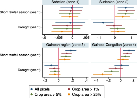
Figure 13. Impact of a bad rainy season on deforestation (threshold: 30% of canopy cover).
Download figure:
Standard image High-resolution imageThe opposite effect of a short rainy season (negative impact of rainy season length) and a lack of seasonal rainfall (positive impact of drought) in the dryer eco-climatic (figure 11) zone must be put into perspective in the light of the scarce presence of trees in this zone (see table 3).
D.3. Rainfall shocks severity: SPI thresholds
The results are robust to different severity of rainfall shocks, corresponding to different SPI threshold. I consider lower thresholds for mild and moderate rainfall shocks (0.5, 0.7) and a higher threshold for a severe rainfall shock (1.5), respectively in figures 14, 15 and 16. The probability of return of a mild rainfall shock is 23.4% for droughts and 23.9% for short rainy seasons (every 4–5 years), the probability of return of a mild rainfall shock is 30.1% for droughts and 31.6% for short rainy seasons (every 3–4 years) and the probability of return of a severe rainfall shock is 5.1% for droughts and 6.5% for short rainy seasons (every 15–20 years).

Figure 14. Impact of a bad rainy season on deforestation (mild droughts and short rainy seasons, both defined by SPI inferior to −0.5).
Download figure:
Standard image High-resolution image
Figure 15. Impact of a bad rainy season on deforestation (moderate droughts and short rainy seasons, both defined by SPI inferior to −0.7).
Download figure:
Standard image High-resolution image
Figure 16. Impact of a very bad rainy season on deforestation (heavy droughts and very short rainy seasons, both defined by SPI inferior to −1.5).
Download figure:
Standard image High-resolution imageExtremely severe droughts (SPI inferior to −2) correspond to events only occurring every 50 years, which seem to small considering the time span of the study period. Similarly, heavy droughts are rare, it may explain why they are found to have a less significant impacts on deforestation in spite of a similar or higher amplitude (see figure 16).
D.4. Deforestation and remoteness: Guinean and Guineo-congolian eco-climatic zones
Here, I show the robustness of heterogeneous results depending on the remoteness and the proportion of crop area, when restricting the sample to the two most humid eco-climatic zones.

Figure 17. Impact of a bad rainy season on deforestation in Guinean and Guineo-congolian eco-climatic zones, depending on the population density (a) and relative remoteness in terms of: time-distance to cities (b) and distance to night-time lights (c).
Download figure:
Standard image High-resolution imageD.5. Standard error adjustment for spatial correlation and serial correlation in panel data
I consider here an alternative estimation method of standard errors that is robust to controlling for spatial correlation and serial correlation in panel data. I employ the recent Stata routine acreg developed by Colella et al (2019) based on Hsiang (2010) and Conley (1999). Details about the statistical regression method are given at the following links:
http://www.fight-entropy.com/2010/06/standard-error-adjustment-ols-for.html.
Table 12 shows the standard errors allowing for spatial correlation of 50 kilometres, and for a serial correlation over 7 consecutive years.
Table 12. Drivers of deforestation: robust to spatial and serial correlation.
| Sahelian zone | ||||
|---|---|---|---|---|
| (1) | (2) | (3) | (4) | |
| Log of deforestation (ares) | All pixels | Crop area 1% | Crop area 5% | Crop area 25% |
| Short rainfall season (year t) | 0.000604 | 0.000287 | 0.000526 | 0.000118 |
| (0.00127) | (0.00126) | (0.00123) | (0.000985) | |
| Drought (year t) | 0.00127 | 0.000466 | 0.000476 | −0.000660 |
| (0.00168) | (0.00153) | (0.00134) | (0.000982) | |
| Observations | 695 381 | 651 852 | 618 260 | 514 976 |
| Sudanian zone | ||||
| Short rainfall season (year t) | 0.0629 | 0.0686 | 0.0598 | 0.0414** |
| (0.0187) | (0.0193) | (0.0175) | (0.0172) | |
| Drought (year t) | −0.0551 | −0.0330 | −0.0200 | −0.00 647 |
| (0.0192) | (0.0192) | (0.0177) | (0.0183) | |
| Observations | 420 669 | 322 382 | 289 284 | 226 527 |
| Guinean zone | ||||
| Short rainfall season (year t) | 0.146 | 0.0893** | 0.0815** | 0.0939 |
| (0.0353) | (0.0369) | (0.0402) | (0.0488) | |
| Drought (year t) | −0.0925** | −0.0437 | −0.0252 | −0.0291 |
| (0.0436) | (0.0452) | (0.0489) | (0.0603) | |
| Observations | 1 124 634 | 587 799 | 476 170 | 315 193 |
| Guineo-congolian zone | ||||
| Short rainfall season (year t) | 0.169 | 0.124 | 0.0852 | 0.0225 |
| (0.0626) | (0.0705) | (0.0781) | (0.0944) | |
| Drought (year t) | −0.0725 | |||
| (0.0673) | (0.0774) | (0.0869) | (0.109) | |
| Observations | 446 481 | 269 808 | 213 130 | 123 924 |


Conley (1999) standard errors in parentheses, allowing for spatial correlation within a 50 km radius and for 7 years serial correlation.* , * , ***


Footnotes
- 1
- 7
- 10
- 12
Pixels with high (low) population density correspond to values higher (lower) than the median value of the log population density (2.6); pixels far (near) from the nearest market are at more (less) than 90 minutes from the nearest city and pixels far (near) from powered settlements are at more (less) than 13.5 km from a detectable night-time light. Regressions are displayed in supplementary tables 9, 10 and 12.
- 2
Dropping approximately 0.033% of the pixel covered with forest.
- 3
These other indices included the number of rainy days, occurrence of heavy rainfall, onset and offset dates, simpler and non standardised cumulative rainfall, other rainfall season definitions an the number of dry spells (7, 10 and 14 d) during the rainfall season.
- 4
i.e. negative variations superior to one standard deviation. Robustness checks with other SPI values thresholds are displayed in section D.3 of supplementary material.
- 5
- 6
- 8
log(X+1), X being the deforestation in ares observed in pixel i and year t. Deforestation is the average forest cover in 2000 of 1 arc-second (approximately 30 m at the equator) pixels lying in 0.05 degree pixels considered as cleared in year t by Hansen et al (2013)'s algorithm. See appendix A.2 of supplementary material for further details about deforestation estimates.
- 9
In the absence of any threshold, any vegetation taller than 5 m in height is considered, which is compatible with the Sahelian zone, where woody cover mainly consist in woody savannah or shrubland.
- 11
The probability of return of the events studied is 15%, meaning that the indices exceed one standard deviation less than once every 6 years.
- 13
i.e. Benin, Burkina Faso, Cameroon, Central African Republic (RCA) Chad, Congo, Democratic Republic of th Congo (DRC), Gabon, Ivory Coast, Niger, Mali, Mauritania and Senegal.
- 14
Version 4 DMSP-OLS Nighttime Lights Time Series, available at:
- 15
The data can be accessed and visualised at the following link access map in 2015.
- 16