

Abstract
The dipole pattern of summer precipitation over the Tibetan Plateau (TP) during 1961–2014 is evaluated based on observations and 18 models provided by the Coupled Model Intercomparison Project Phase 6. Of the 18 models, 10 can capture the opposite variation characteristics in the south and north TP. Observational data reveals that the south–north seasaw of TP summer precipitation is essentially driven by a Rossby wave propagating from the Western Europe to East Asia, which is associated with North Atlantic oscillation (NAO). The models successfully simulated the dipole pattern that is closely related to the reproduction of the NAO–TP relationship. Further analysis demonstrates that the reliable simulations of horizontal dynamic processes of moisture transport, which is linked to the NAO–TP relationship, highly contributes to their success in reproducing the dipolar pattern of TP summer precipitation. While unrealistic local vertical circulation and evaporation simulation lead to the failed reproductions. These findings provide significant information for model development and future climate change projections.
Export citation and abstract BibTeX RIS

Original content from this work may be used under the terms of the Creative Commons Attribution 4.0 license. Any further distribution of this work must maintain attribution to the author(s) and the title of the work, journal citation and DOI.
1. Introduction
The Tibetan Plateau (TP), known as the 'Third Pole of the word', has a significant impact on global weather and climate systems through dynamic and thermal effects (Wu et al 2007). The TP is also the origin of many Asian rivers, e.g. the Yellow River, Yangtze River and Mekong River, leading to it being called the 'Asian water tower' (Xu et al 2008). The summer precipitation over the TP is abundant and accounts for more than half of the total annual rainfall changes in amount (Feng and Zhou 2012), and has experienced significant changes in recent decades (Yang et al 2014, Yao et al 2019). The variations of the TP precipitation are critically important for the hydrological cycle and ecology balance. Thus, it is of great significance to understand the mechanisms and moisture transport processes of the summer TP precipitation.
The summer precipitation of TP dominantly shows an antiphase between the south and north TP at interannual variability (Liu and Yin 2001, Liu et al 2015). The variation of summer TP precipitation is not only influenced by the Asian monsoon circulation, but also affected by the teleconnection associated with the North Atlantic Ocean as well as the North Atlantic oscillation (NAO), the Pacific Ocean and the Indian Ocean (Bothe et al 2010, Gao et al 2013, Hu et al 2016, Sun et al 2020). Wang et al (2017) revealed that the interannual variation of precipitation over the south TP is related to the moisture from western boundary and is primarily modulated by westerlies and strong NAO. With respect to atmospheric moisture transport, many studies have documented the different moisture sources of the TP and their variations on different timescales (Curio et al 2015, Dong et al 2016, Zhang et al 2017a, Zhou et al 2019). Zhang et al (2019) examined that in terms of climatology, the moisture in the north TP mainly came from Europe, whereas that in the south TP is associated with the Indian Ocean. Furthermore, the summer TP precipitation is dominantly explained by the dynamic process of atmospheric moisture budget, which is due to circulation changes, and less attribute to the thermodynamic process that is associated with specific humidity anomalies (Gao et al 2014, Wang et al 2017, Zhang et al 2017b).
Global coupled climate models have been extensively explored to understand variations in climate systems and to project future climate changes. Based on the Coupled Model Intercomparison Project phase 5 (CMIP5), global climate models have many discrepancies for precipitation simulation. For instance, CMIP5 models overestimate the annual mean precipitation over the TP, especially for the southeastern regions (Chen and Frauenfeld 2014, Jiang et al 2016, Yue et al 2016). Furthermore, only half of the CMIP5 models could capture the observed seasonal pattern of TP precipitation (Su et al 2013, Hu et al 2014). The seesaw pattern between the TP precipitation and East Asian summer monsoon, which is observed on interannual timescale, is also poorly reproduced (Duan et al 2013). The large biases of CMIP5 models regarding TP precipitation may be linked to the coarse resolution, subgrid-scale physics, inaccurate simulation of circulation and complex terrains (Duan et al 2013, Zhang and Li 2016, Chen et al 2017, Salunke et al 2019). Recently, CMIP6 has issued the outputs simulated by state-of-the-art models in the worldwide. Most CMIP6 models have improved model resolution, optimized physical schemes, and included additional biochemical process in the earth system (Eyring et al 2016). More advanced models are provided to achieve more reliable precipitation simulations and future projections (Chen et al 2020, Park et al 2020, Zhu et al 2020). However, few works have focused on the simulation of TP regions. Therefore, it is of great necessity to evaluate the performance of CMIP6 models in reproducing the TP precipitation, particularly the interannual variation in summer.
In this study, we examined the simulation of interannual dipolar pattern of summer TP precipitation in CMIP6 models. Then, how well the CMIP6 models capture the teleconnection relationship between the summer TP precipitation and NAO is discussed. The physical process associated with atmospheric moisture budget is also diagnosed. The aim of this study is to assess the ability of CMIP6 models in reproducing the variability of summer TP precipitation and the underlying physical processes, which provides useful insights into model development and future climate changes projection.
2. Data and methods
2.1. Datasets
The datasets used included the following: (a) monthly precipitation grid dataset of 0.5° × 0.5° horizontal resolution for the period of 1961–2014, distributed across TP regions provided by the Climate Data Center, China Meteorological Administration. (b) Monthly reanalysis data for geopotential height, wind, vertical velocity, specific humidity and evaporation on 2.5° × 2.5° horizontal resolution for 1961–2014 period, obtained from the National Center for Atmospheric Research (NCEP/NCAR) (Kalnay et al 1996), and 1° × 1° horizontal resolution in 1979–2014 period provided by the European Center for Medium-Range Weather Forecasts (ERA-Interim, Dee et al 2011). The observational and reanalysis datasets are called 'observation' in the present study. (c) The monthly historical simulation for 18 CMIP6 models from 1961–2014 is used in this study. The model outputs are interpolated into the same resolution to compare with the observation datasets. More detail information for the 18 CMIP6 models is in table 1 and can also be found at https://esgf-node.llnl.gov/search/cmip6/.
Table 1. Model name, institute ID, latitude and longitude numbers of each model used in this study.
| No. | Model name | Model full name | Institution ID | Lat × Lon |
|---|---|---|---|---|
| 1 | ACCESS-CM2 | Australian Community Climate and Earth System Simulator | CSIRO/Australia | 144 × 192 |
| 2 | ACCESS-ESM1-5 | Earth Systems Model version of ACCESS | CSIRO/Australia | 144 × 192 |
| 3 | BCC-CSM2-MR | Beijing Climate Center Climate System Model | BCC/China | 160 × 320 |
| 4 | CAMS-CSM1-0 | The Climate System Model of the Chinese Academy of Meteorological Sciences | CAMS/China | 160 × 320 |
| 5 | CESM2 | Community Earth System Model version 2 | NCAR/USA | 192 × 288 |
| 6 | EC-Earth3 | European community Earth-System Model | EC-Earth-Consortium/EU | 256 × 512 |
| 7 | EC-Earth3-Veg | European community Earth-System Model with interactive vegetation module | EC-Earth-Consortium/EU | 256 × 512 |
| 8 | FGOALS-f3-L | Flexible Global Ocean-Atmosphere-Land System model | CAS/China | 180 × 288 |
| 9 | FIO-ESM-2-0 | First Institute of Oceanography Earth System Model version 2.0 | FIO-QLNM/China | 192 × 288 |
| 10 | GISS-E2-1-G | Goddard Institute for Space Studies Earth System Model-G | NASA-GISS/USA | 90 × 144 |
| 11 | GISS-E2-1-H | Goddard Institute for Space Studies Earth System Model-H | NASA-GISS/USA | 90 × 144 |
| 12 | INM-CM5-0 | Russian Institute for Numerical Mathematics Climate Model Version 5 | INM/Russia | 120 × 180 |
| 13 | KACE-1-0-G | Korea Meteorological Administration Advanced Community Earth-system model | KMA/Korea | 144 × 192 |
| 14 | MIROC6 | MIROC Consortium model version 6 | MIROC/Japan | 128 × 256 |
| 15 | MPI-ESM1-2-LR | Max Planck Institute Earth System Model-LR | MPI-M/Germany | 96 × 192 |
| 16 | NESM3 | Nanjing University of Information Science and Technology Earth System Model version 3.0 | NUIST/China | 96 × 192 |
| 17 | NorESM2-MM | Norwegian Earth System Model version 2MM | NCC/Norway | 192 × 288 |
| 18 | SAM0-UNICON | Seoul National University Atmosphere Model version 0 with a Unified Convection Scheme | SNU/Korea | 192 × 288 |
2.2. Atmospheric moisture budget analysis
The regional precipitation is generally connected with evaporation and moisture transport. The anomalous moisture budget (Chou et al 2009, Seager et al 2010) is expressed as follows:

where q is the specific humidity, P is the precipitation, E is the evaporation, V is the horizontal wind vector (u, v),  is the vertical pressure velocity.
  represents a vertical integration from surface to 300 hPa. The time variation of specific humidity term
  can be neglected on the seasonal mean timescale.
A variable is decomposed into its time mean (overbar) and interannual anomalies (prime) and non-interannual components, the anomalous interannual moisture transport term in (1) can be expressed as:
where term  and term
  represent the horizontal and vertical moisture advection. The dynamic terms in horizontal and vertical terms are
  and
and  . The thermodynamic terms are
  and
and  , respectively. Reside is represent the nonlinear interaction part. Term
  ,
,  and residue are very small terms and, hence, are ignored in this study.
3. Results
3.1. Dipole pattern of Tibetan summer precipitation in CMIP6 models
Figure 1(a) plots the first empirical orthogonal function (EOF) pattern of the observation. It demonstrates a dipole pattern in the south and north TP with a 21% variance being explained. The EOF1 pattern of the CMIP6 models are shown in figures 1(b) and (s). There are large differences among the CMIP6 models and the variances range between 14% and 23%. According to the pattern correlation coefficients of EOF1 between the observation and models, the models can be categorized into two groups. (a) Better group (BG) models, with correlation coefficients larger than 0.5, comprising CAMS-CSM1-0, CESM2, EC-Earth3, EC-Earth3-Veg, FIO-ESM-2-0, GISS-E2-1-G, KACE-1-0-G, MIROC6, NESM3, and SAM0-UNICON. (b) Worse group (WG) models, with pattern coefficients smaller than 0.5, involving ACCESS-CM2, ACCESS-ESM1-5, BCC-CSM2-MR, FGOALS-f3-L, GISS-E2-1-H, INM-CM5-0, MPI-ESM1-2-LR, and NorESM2-MM. Besides the pattern correlation coefficients of EOF1, we also consider the latitude of the Tanggula Mountains separating the south and north TP at 33° N–34° N. All the BG models reproduce the dipole pattern and, in each model, the center of the pattern is located over the central-eastern TP, similar to observation. However, the EOF1 pattern shows strong differences across the WG models. For example, the centers are simulated in the western TP in ACCESS-CM2 and BCC-CSM2-MR, and the separating latitude is north of the Tanggula Mountains.
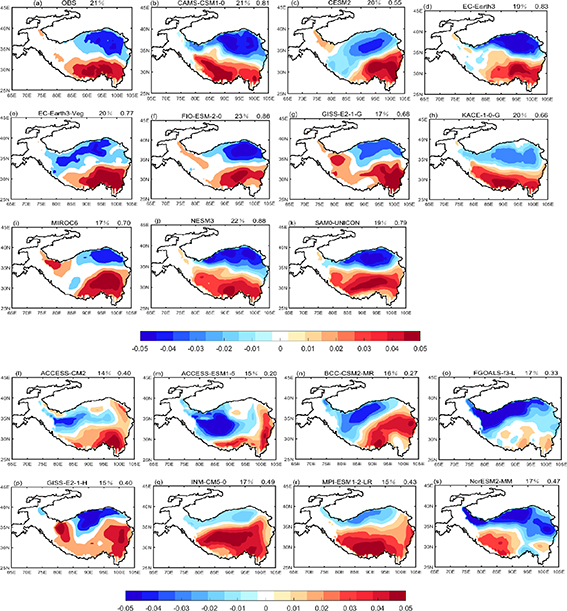
Figure 1. Spatial pattern of the first EOF mode of summer precipitation over the TP for (a) observation; (b)–(k) the results for CMIP6 models in the BG; (i)–(s) the results for CMIP6 models in the WG. The spatial correlation coefficient of first EOF between the observation and CMIP6 models are plotted at top-right corners.
Download figure:
Standard image High-resolution imageFigure 2 displays the variation of summer precipitation averaged over the south TP (27° N–33° N, 85° E–105° E) and north TP (34° N–39° N, 85° E–105° E) by each model and the ensemble means of the BG models (figure 2(a)) and WG models (figure 2(b)). Both the south and north TP precipitation manifest an interannual variation during 1961–2014. In the BG models, the precipitation over the south TP and north TP demonstrates the opposite variation with a correlation coefficient of −0.46, consistent with the EOF1 pattern. However, the correlation is only −0.11 for the WG models, much lower than the significant test. The results verify the well simulation of the dipole pattern of TP summer precipitation in the BG models.
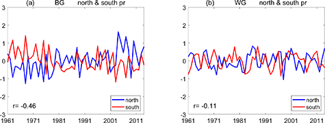
Figure 2. (a) The time series of the anomalies of areal precipitation (unit, mm d−1) averaged in south (red line) and north (blue line) TP from 1961 to 2014 by CMIP6 models ensemble-mean in the BG; (b) the same as in (a) but for CMIP6 models ensemble-mean in the WG.
Download figure:
Standard image High-resolution image3.2. Influence of the North Atlantic oscillation
The interannual variation of precipitation over the TP is dominantly influenced by the moisture transport from the western boundary, which is associated with the NAO (Gao et al 2013, Liu et al 2015, Wang et al 2017). In this section, we focus on the teleconnection between the NAO and TP precipitation variation and assess the models' performance when simulating this relationship.
Figures 3(a) and (c) illustrate the regression fields of sea level pressure (SLP) anomalies against the PC1 (time series of principal component) of TP summer precipitation in observation, ensemble-mean BG models and WG models, respectively. In observation, there are high SLP anomalies in Iceland and low SLP anomalies in Azores. This north–south opposite pattern over the North Atlantic is related to the negative NAO phase (Watanabe et al 1999, Pan 2005). Meanwhile, low pressure anomalies manifest over the south TP, which favors the enhancement of local precipitation. The BG models could successfully reproduce the dipolar SLP pattern over the North Atlantic sector exactly consistent with the observation. However, in the WG models, the SLP anomalies are inverse to the observation and BG models. Although weaker low anomalies appear in the TP, they may not be associated with the NAO.

Figure 3. Regression fields of the sea level pressure anomalies (shading; Pa) against PC1 for (a) observation; (b) BG models; (c) WG models. The dotted areas indicate the 95% confidence level. (d)–(f) The same as (a)–(c), but for 200 hPa geopotential height anomalies (shading; gpm) and wind anomalies (vector; m s−1). Only where exceeding the 95% significant level are displayed. The green line displays the Tibetan Plateau.
Download figure:
Standard image High-resolution imageTo further demonstrate the impact of NAO on TP summer precipitation, figures 3(d) and (f) depict the regression anomalies of geopotential height and wind at 200 hPa against PC1. In observation, there is an evident Rossby wave train propagating from northwestern Europe to southern TP, which resembles that stimulated by the negative NAO phase (Liu et al 2015, Wang et al 2017). Such wave train causes a strong anticyclone over the south TP, enhancing the divergence in the upper troposphere and providing beneficial conditions for abnormal precipitation. This wave train connects the NAO and TP precipitation, suggesting the importance of western boundary downstream moisture transport. The regression anomalies of the SLP pattern and associated Rossby waves at 200 hPa are also clearly seen by using the ERA-interim reanalysis data for the observation (figure S1 (available online at stacks.iop.org/ERL/16/014047/mmedia)). In the BG models, the Rossby wave related to NAO anomalies is closely similar to that of the observation, indicating the successful simulation of the NAO–TP relationship. In contrast, the wave trains in the WG models are much weaker and are not reproduced as the NAO phase.
In general, the BG models could simulate the dipolar SLP anomalies and Rossby waves associated with NAO anomalies, which contribute to reproduce the dipole pattern of TP precipitation. However, this process is not captured in the WG models. The above analysis confirms that the simulation of the dipole pattern of summer TP precipitation is exactly related to the reproduction of the teleconnection relationship between the NAO and TP.
A realistic NAO in terms of structure and variability may be vital for reproducing the TP summer precipitation pattern. Thus, we have checked the summer NAO pattern in the BG and WG models (figure S2). The spatial extent and intensity of the summer NAO are weaker than the winter NAO, and the center is located further north to the Western Europe (Folland et al 2009). In the BG model, the NAO pattern is well reproduced, which is similar to the observation. However, the SLP anomalies exhibit a tripolar pattern over North Atlantic regions in the WG models. That means the WG models fail to capture the summer NAO pattern, and thus the unrealistic impact of NAO on TP precipitation.
It is interesting to note that the weak low surface pressure and high pressure at 200 hPa in the WG models are also favorable for precipitation over TP. However, they are not related to NAO and downstream moisture transport. It also implies that the NAO may not the only reason for the anomalous precipitation over TP. According to the moisture budget in equation (1), the regional precipitation anomalies may both influenced by the remote moisture transport and local evaporation. For the dipole pattern of TP precipitation, the horizontal moisture transport is dominantly related to the NAO in observation and BG models. However, the unrealistic anomalous local circulation and evaporation could also cause the precipitation changes, which may affect the failed simulation in the dipole pattern of TP precipitation for the WG models. Further detailed analysis will be discussed in the next section.
3.3. Diagnosis of atmospheric moisture budget
We diagnose the atmospheric moisture budget to demonstrate the dynamic and thermodynamic process contributions to the dipole TP summer precipitation. In observation, the dynamic component could explain large majority variance of the TP moisture transport, whereas the thermodynamic and evaporation contributions are the much smaller on interannual timescale (Wang et al 2017, Zhang et al 2017a). This implies that the variations in atmospheric circulation play a more important role in the water vapor transport of summer TP precipitation than the specific humidity changes.
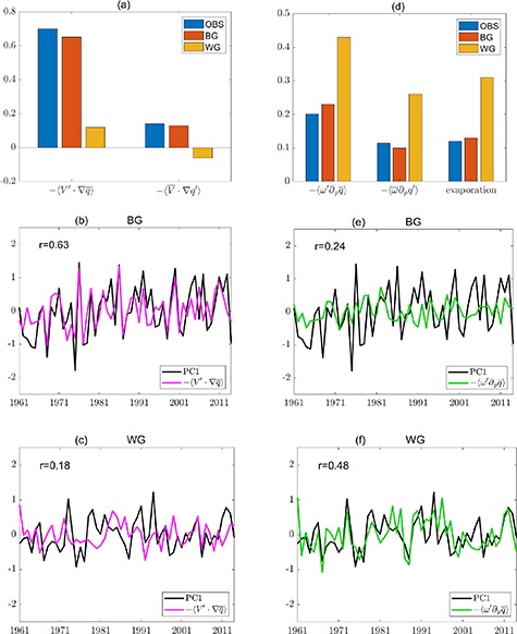
Figure 4(a) shows the regression anomalies of the horizontal components of moisture convergence against PC1 averaged over the south TP (27° N–33° N, 85° E–105° E) for observation, BG ensemble-mean and WG ensemble-mean. In observation, the dipolar pattern of TP precipitation is dominated by the horizontal dynamic term ( ), which is substantially linked to the NAO influence and western boundary moisture transport. The horizontal thermodynamic term (
 ) contributes much less to TP precipitation. Thus, we focus on the dynamic part of the moisture transport. In the BG models, the horizontal dynamic term resembles that of the observation. However, the WG models simulate much smaller values than the observation and BG models. In addition, the correlation between the ensemble-mean PC1 and horizontal dynamic term in the BG models can be reached to 0.63 at 99% significant level (figure 4(b)), while it is only 0.18 in the WG models (figure 4(c)). This suggests that the WG models could not accurately simulate the dynamic process of moisture transport related to the dipole pattern of TP precipitation, consistent with their inability to reproduce the NAO–TP relationship. Better simulation of the dynamic process indicates a realistic reproduction of atmosphere circulations affecting the water vapor transport, and thus the dipolar pattern of the TP summer precipitation.
Figure 4. (a) Regression of  and
and  anomalies against the PC1 averaged over the south TP (27° N–33° N, 85° E–105° E) for observation, BG ensemble-mean and WG ensemble-mean. (b) Time series of the PC1 and
  anomalies averaged over south TP in BG ensemble-mean; (c) the same as (b) but for the WG ensemble-mean; (d) regression of
  ,
,  and evaporation anomalies against the PC1 averaged over the south TP for observation, BG ensemble-mean and WG ensemble-mean. (e) Time series of the PC1 and
  anomalies averaged over south TP in BG ensemble-mean; (f) the same as (e) but for WG ensemble-mean. All variables of units are mm d−1.
Download figure:
Standard image High-resolution image
The vertical components of moisture convergence and evaporation anomalies are given in figure 4(d). In the observation and BG models, the vertical process and evaporation anomalies have less impact on the water vapor transport than the horizontal moisture transport. In contrast, they are simulated to be much more significant in the WG models. Though the individual models may behave different performance, the WG models simulate much larger biases of local vertical circulation and evaporation anomalies, especially in the south TP regions (figures S3 and S4). The correlation between the ensemble-mean PC1 and vertical dynamic term ( ) is only 0.24 in the BG models (figure 4(e)), while it is twice as large (0.48) in the WG model (figure 4(f)). Furthermore, the evaporation anomalies in the WG models also have larger deviation than those in observation and BG models, especially in the south TP regions. That means the major contribution of the TP precipitation anomalies in the WG models can be attributed to the anomalous local vertical circulation and evaporation. The large deviations in the horizontal and vertical dynamic components of moisture convergence suggest the false simulation in water vapor transport of the summer TP precipitation, which further affects the reproduction of precipitation over the south and north TP in the WG models.
4. Summary and discussion
The present study investigates the dipolar pattern of summer precipitation in TP regions based on the observations and 18 CMIP6 models. In observation, the summer precipitation in TP is characterized as an opposite variation in south and north TP. This dipolar pattern is primarily driven by Rossby wave trains propagating from the North Atlantic Ocean to East Asia. The wave trains cause an anomalous anticyclone in the upper troposphere, increasing the divergence, which favors for the precipitation in the south TP.
Of the 18 CMIP6 models, 10 can capture the dipole pattern of summer TP precipitation. According to the pattern correlation coefficient of EOF1 and the latitude of Tanggula Mountains, we divide the models into two groups. The BG models could simulate a realistic dipole pattern that closely resembles to the observation, whereas it is not well reproduced in WG models. Further analysis reveals that the BG models capture the NAO–TP relationship as well as the wave trains from the Western Europe to East Asia. In contrast, the WG models fail to achieve this teleconnection.
The water vapor convergence is further discussed based on the atmosphere moisture budget. For observational data, the dynamic process largely contributes to the summer TP precipitation. The positive impact of dynamics process is reliable reproduced in the BG models. However, the WG models capture much weaker horizontal dynamic process. Further, the dramatic local vertical circulation and evaporation processes have more impact on the TP precipitation in the WG models. Thus, the success of BG models reproducing the dipolar pattern of summer TP precipitation is attributed to the realistic simulation of the dynamic process associated with moisture transport. While the failure of the WG models is mainly related to the unrealistic local vertical circulation and evaporation simulation.
It is noted that the TP precipitation variation is complicated and changeable, and latent heating releasing from precipitation may influence the 'pumping effect' and related circulations (Wu et al 2017, He et al 2019). The moisture source of TP precipitation could be associated both with the westerlies and monsoon (Pan et al 2019, Zhang et al 2019, Zhou et al 2019). However, different mode variations of TP precipitation may have distinguished mechanisms at multi-timescales. Our findings emphasized the NAO–TP relationship, as well as the underlying horizontal dynamic moisture transport for the dipole pattern of summer TP precipitation at interannual timescale, both in observation and models. These findings are beneficial for understanding and developing the simulation of TP precipitation. The different abilities of BG and WG models in reproducing the dipole pattern of summer TP precipitation are also likely connected to the simulations of the interaction between atmosphere and land surface component. The development of land surface model (e.g. soil moisture transportation and land over phenology) may have potential to improve the coupled model performance in capturing the two items. Additionally, the resolutions of the global climate models are still rougher than the regional models, resulting in the complex terrain may be neglected. Thus, in order to simulate more detailed TP precipitation, the dynamic downscaling work needs to be taken into consideration in the future.
Acknowledgments
We thank anonymous reviewers for comments and suggestions that have substantially improved the manuscript. This work was jointly supported by the Second Tibetan Plateau Scientific Expedition and Research (STEP) program (Grant No. 2019QZKK0201), the National Natural Science Foundation of China (Grant Nos. 41571062, 41675067 and 41701592) and the Postdoctoral Science Foundation of China (Grant No. 2019M663616). The monthly precipitation data was provided by the China Meteorological Administration for academic use from http://data.cma.cn/en/?r=data/index&cid=6d1b5efbdcbf9a58. The NCEP/NCAR monthly reanalysis data could be freely obtained from the website www.esrl.noaa.gov/psd/data/gridded/data.ncep.reanalysis.html. The ERA-Interim monthly reanalysis data could be freely downloaded from https://apps.ecmwf.int/datasets/data/interim-full-moda/levtype=sfc/. The CMIP6 model data was accessed from https://esgf-node.llnl.gov/search/cmip6/.
Data availability statement
All data that support the findings of this study are included within the article (and any supplementary files).