

Abstract
Nutrient and sediment transport exhibit strong spatial and temporal inequality, with a small percentage of locations and events contributing to the vast majority of total annual loads. The processes for determining how to reduce total annual loads at a watershed scale often target spatial, but not temporal, components of inequality. We introduce a framework using Lorenz Inequality and corresponding Gini Coefficient to quantify the temporal inequality of nutrient and sediment transport across the Chesapeake Bay watershed. This long-impaired, 166 000 km2 watershed has been federally mandated since 2010 to continually reduce nutrient and sediment loads reaching the Bay. Data were obtained for 108 sites in the Chesapeake Bay's non-tidal network from 2010 to 2018. The Lorenz Inequality and Gini Coefficient analyses were conducted using daily-scale data for flow and loads of total nitrogen (TN), total phosphorus (TP), and total suspended sediment (TSS) at each gaging station. We leverage these results to create a 'temporal targeting framework' that identifies periods of time and corresponding flow conditions that must be targeted to achieve desired or mandated load reduction goals across the watershed. Among the 108 sites, the degree of temporal inequality for TP and TSS (0.37–0.98) was much greater than for flow and TN (0.29–0.77), likely due to the importance of overland versus baseflow in the transport pathways of the respective constituents. These findings stress the importance of informed design and implementation of best management practices effective in 'hot moments,' and not just 'hot spots,' across impaired watersheds to achieve and maintain water quality restoration goals. The 'temporal targeting framework' detailed in this manuscript provides a useful and convenient method for watershed planners to create low- and high-flow load targeting tables specific to a watershed and constituent.
Export citation and abstract BibTeX RIS

Original content from this work may be used under the terms of the Creative Commons Attribution 4.0 license. Any further distribution of this work must maintain attribution to the author(s) and the title of the work, journal citation and DOI.
1. Introduction
Water quality degradation of coastal water bodies due to the presence of excess nutrients is a leading global environmental concern (Selman et al 2008, Gilbert et al 2010, Sutton et al 2011, 2013). More than 400 coastal areas around the world are classified as either eutrophic or hypoxic, with only 13 classified as 'in recovery' (Selman et al 2008). Agricultural activities are common contributors of excess nutrients contributing to degraded water quality, with wastewater, atmosphere deposition, and urban stormwater as other contributors (Mateo-Sagasta et al 2017).
The Chesapeake Bay is the largest estuary in the United States and the third largest in the world, with a watershed spanning 166 000 km2 across six states and the District of Columbia. The watershed is home to more than 18 million people and has a land-to-water ratio of 14:1, which is the largest ratio of a coastal estuary in the world (Kemp et al 2005, National Park Service 2018, Chesapeake Bay Program 2020a, Maryland Department of the Environment, n.d.). The result is a substantial effect of land use activities on water quality conditions. Excess nutrients and sediment have degraded the Bay's water quality for decades, leading to the establishment of a total maximum daily load (TMDL) by the United States Environmental Protection Agency (USEPA) in 2010. The TMDL mandates that each state implements control measures to reduce nitrogen, phosphorus, and sediment loads into the Bay by 25%, 24%, and 20% respectively, to restore the Bay's water quality by 2025 (USEPA 2010). Although best management practice (BMP) adoptions have certainly helped restoration efforts, overall water quality improvements in the Bay have been difficult to show (Zhang et al 2018).
The Chesapeake Bay Program (2020b) estimates that agricultural land uses contribute 42%, 55%, and 60% of the excess total nitrogen (TN), total phosphorus (TP), and total suspended sediment (TSS) reaching the Bay. Clearly, further reductions in nutrient and sediment losses are necessary to achieve the established water quality goals. Except for large confined animal feeding operations that are regulated as point sources under the Clean Water Act, public policies for reducing agricultural nonpoint source pollution rely on voluntary adoption of BMPs (Ribaudo and Shortle 2019). Although some adoption occurs without public sector financial assistance, cost-sharing subsidies offered through the USDA Environmental Quality Incentive Program and other programs are crucial to significant BMP implementation. Given limited federal and state budgets, targeting resources spatially to locations that contribute disproportionately large pollutant quantities is essential for maximizing the effectiveness of public and private investments in pollution control (Shortle et al 2012, Ribaudo and Shortle 2019). By calculating area-normalized loads, hot spots can be identified as the locations within a watershed that have the highest loads per unit area. In this way, decision makers can direct resources to a relatively small number of places, knowing that implementation of BMPs in those locations will achieve a higher impact on load reduction than placing the same resources and BMPs in areas elsewhere. Research has shown that spatially targeting BMP adoption leads to larger load reduction at the watershed scale (e.g. Gitau et al 2006, Ghebremichael et al 2013, Geng et al 2019, Amin et al 2020, Karki et al 2020).
It is also important to recognize and manage temporal inequalities, or hot moments, so that resources can be targeted based on both spatial and temporal inequalities. Unfortunately, no uniform metric for describing temporal inequality is widely adopted, despite the prevalence of temporal inequality documentations in both small and large watersheds. Richards et al (2007) reported the export of more than 70% of TP, dissolved reactive phosphorus, nitrate, and SS loads occurred during approximately one-third of the time in four predominantly agricultural catchments in the Lake Erie Basin that ranged several orders of magnitude in size (88–16 000 km2). Royer et al (2006) found that almost all of the nutrient loads for agricultural catchments in Illinois spanning a four-fold range in area were exported when the flowrate was greater than the median value. Furthermore, the size of the dead zone in the Gulf of Mexico has been found to be directly correlated to the precipitation in the Midwestern United States, suggesting that high-flow events deliver the majority of nutrient loads to the Gulf (Donner and Scavia 2007). For the Susquehanna River, the largest tributary to Chesapeake Bay, it was reported that Tropical Storm Lee alone exported 31%, 61%, and 78% of TN, TP, and TSS, respectively, in the entire 2011 water year (Hirsch 2012). Despite the documented importance of temporal inequality in the export dynamics of constituent loads, there is currently no uniform method for assessing, quantifying, or leveraging this information to better inform the adoption of appropriate BMPs for more targeted management.
The goal of this paper is to develop a new framework for BMP design and implementation that links specific flow events to the temporal inequality of nutrient and sediment transport in the Chesapeake Bay watershed. Here, we adopt Lorenz Inequality analysis, which is commonly used in economics to quantify income inequality within a population, and apply it to time series data for nutrient and sediment loads for monitoring stations in the Chesapeake Bay's non-tidal network (NTN). Lorenz Inequality results, along with the Gini Coefficient, allow us to quantify the temporal inequality of flow, TN, TP, and TSS for 108 locations across the Bay watershed. We then link the temporal inequality of each constituent to specific flowrates using flow duration curves (FDCs), which allows us to identify the flowrates that occur when large portions of loads are exported. The information obtained from this analysis is then used to develop a decision-making framework that can inform design and implementation of agricultural BMPs to more effectively target 'hot moments' based on the load reduction goals required by the Bay's TMDL (USEPA 2010). This decision-making framework can allow land managers to understand the critical time periods for achieving load reduction goals, and the potential consequences associated with failure to treat high-flow events effectively. Additionally, the framework provides land managers with a convenient and flexible method of identifying different ways to achieve the same load reduction goal (e.g. 25%) under either low or high-flow conditions. The results of this approach have implications for farmers, practitioners, researchers, and policy makers in the Chesapeake region, with an approach that is easily transferable to other watersheds. It is our hope that this temporal targeting approach is implemented with spatial targeting of BMPs to help achieve water quality restoration goals in impaired watersheds worldwide.
2. Methods
2.1. Study sites
The Chesapeake Bay's NTN is a network of water quality and quantity data collected by the United States Geological Survey (USGS) across the Chesapeake Bay watershed at more than 100 locations (Moyer and Langland 2020). The USGS and partner agencies process the data and provide discharge and estimated loads for nutrients and sediment for public use (see: https://cbrim.er.usgs.gov/index.html). Load and discharge data at a daily time scale were obtained from the database over an 8 year period (by water year; October–September) from 2010–2018 for 108 sites that had discharge, TN, TP, and TSS (table 1). Drainage areas for the selected sites ranged from less than 2 km2 to as large as sim 70 000 km2. Twenty of the watersheds were dominantly agricultural (row cropped fields and pasture >50% of the drainage area), 10 were dominantly (>50%) developed, and 46 were dominantly forested. The remaining 32 sites were mixed use, with no one dominant land cover. The distribution of dominant land uses across the study sites enabled us to assess temporal inequality of nutrient and sediment loading as functions of watershed size and land use.
Table 1. Gaging stations, drainage areas, land uses, and Gini Coefficients for 108 studied sites in the Chesapeake Bay Watershed. Land use is based on USGS 2016 National Land Cover Data (www.mrlc.gov/data/nlcd-2016-land-cover-conus).
| USGS station ID | Site name | Drainage area (km2) | % Forest | % Developed | % Agriculture | GQ | GTN | GTP | GTSS |
|---|---|---|---|---|---|---|---|---|---|
| 1486000 | Manokin Branch near Princess Anne, MD | 12.4 | 13 | 9 | 31 | 0.58 | 0.65 | 0.76 | 0.84 |
| 1487000 | Nanticoke River near Bridgeville, DE | 195.3 | 7 | 19 | 57 | 0.39 | 0.35 | 0.58 | 0.72 |
| 1488500 | Marshyhope Creek near Adamsville, DE | 121.2 | 8 | 4 | 56 | 0.52 | 0.49 | 0.80 | 0.83 |
| 1491000 | Choptank River near Greensboro, MD | 292.7 | 13 | 5 | 59 | 0.55 | 0.54 | 0.72 | 0.76 |
| 1491500 | Tuckahoe Creek near Ruthsburg, MD | 220.7 | 13 | 5 | 66 | 0.51 | 0.43 | 0.72 | 0.78 |
| 1493112 | Chesterville Branch near Crumpton, MD | 15.9 | 14 | 5 | 62 | 0.33 | 0.25 | 0.89 | 0.94 |
| 1493500 | Morgan Creek near Kennedyville, MD | 32.9 | 4 | 4 | 83 | 0.46 | 0.47 | 0.81 | 0.95 |
| 1495000 | Big Elk Creek at Elk Mills, MD | 133.6 | 34 | 24 | 39 | 0.45 | 0.48 | 0.88 | 0.96 |
| 1502500 | Unadilla River at Rockdale, NY | 1346.8 | 62 | 5 | 29 | 0.50 | 0.54 | 0.79 | 0.88 |
| 1503000 | Susquehanna River at Conklin, NY | 5780.9 | 63 | 14 | 16 | 0.49 | 0.55 | 0.79 | 0.90 |
| 1515000 | Susquehanna River near Waverly, NY | 12 362.0 | 53 | 8 | 34 | 0.49 | 0.51 | 0.72 | 0.86 |
| 1529500 | Cohocton River near Campbell, NY | 1217.3 | 65 | 6 | 24 | 0.55 | 0.58 | 0.79 | 0.88 |
| 1531000 | Chemung River at Chemung, NY | 6490.5 | 57 | 14 | 25 | 0.59 | 0.61 | 0.78 | 0.91 |
| 1531500 | Susquehanna River at Towanda, PA | 20 194.1 | 44 | 11 | 37 | 0.51 | 0.54 | 0.74 | 0.86 |
| 1534000 | Tunkhannock Creek near Tunkhannock, PA | 992.0 | 53 | 8 | 32 | 0.57 | 0.69 | 0.84 | 0.93 |
| 1536500 | Susquehanna River at Wilkes-Barre, PA | 25 796.3 | 33 | 50 | 8 | 0.51 | 0.57 | 0.82 | 0.93 |
| 1540500 | Susquehanna River at Danville, PA | 29 059.7 | 37 | 8 | 47 | 0.50 | 0.57 | 0.75 | 0.87 |
| 1542500 | West Branch Susquehanna River at Karthaus, PA | 3786.6 | 80 | 3 | 14 | 0.49 | 0.58 | 0.79 | 0.83 |
| 1549700 | Pine Creek below Little Pine Creek near Waterville, PA | 2444.9 | 80 | 6 | 11 | 0.56 | 0.71 | 0.85 | 0.91 |
| 1549760 | West Branch Susquehanna River at Jersey Shore, PA | 13 532.7 | 48 | 14 | 33 | 0.50 | 0.55 | 0.78 | 0.88 |
| 1553500 | West Branch Susquehanna River at Lewisburg, PA | 17 733.6 | 35 | 16 | 40 | 0.51 | 0.55 | 0.76 | 0.86 |
| 1553700 | Chillisquaque Creek at Washingtonville, PA | 13.0 | 32 | 6 | 62 | 0.61 | 0.72 | 0.90 | 0.97 |
| 1554000 | Susquehanna River at Sunbury, PA | 47 396.8 | 47 | 14 | 25 | 0.47 | 0.55 | 0.71 | 0.85 |
| 1555000 | Penns Creek at Penns Creek, PA | 779.6 | 52 | 6 | 37 | 0.52 | 0.58 | 0.78 | 0.87 |
| 1555500 | East Mahantango Creek near Dalmatia, PA | 419.6 | 41 | 7 | 51 | 0.55 | 0.66 | 0.74 | 0.95 |
| 1556000 | Frankstown Branch Juniata River at Williamsburg, PA | 753.7 | 63 | 6 | 30 | 0.49 | 0.47 | 0.57 | 0.87 |
| 1558000 | Little Juniata River at Spruce Creek, PA | 569.8 | 61 | 8 | 31 | 0.46 | 0.40 | 0.58 | 0.89 |
| 1562000 | Raystown Branch Juniata River at Saxton, PA | 1958.0 | 81 | 6 | 10 | 0.58 | 0.59 | 0.83 | 0.93 |
| 1565000 | Kishacoquillas Creek at Reedsville, PA | 424.8 | 50 | 15 | 34 | 0.48 | 0.44 | 0.59 | 0.83 |
| 1567000 | Juniata River at Newport, PA | 8686.8 | 62 | 9 | 25 | 0.51 | 0.57 | 0.73 | 0.85 |
| 1568000 | Sherman Creek at Shermans Dale, PA | 536.1 | 70 | 7 | 21 | 0.57 | 0.65 | 0.86 | 0.94 |
| 1570000 | Conodoguinet Creek near Hogestown, PA | 1217.3 | 39 | 20 | 34 | 0.48 | 0.47 | 0.76 | 0.89 |
| 1 570 500 | Susquehanna River at Harrisburg, PA | 62 418.7 | 21 | 42 | 13 | 0.45 | 0.55 | 0.72 | 0.82 |
| 1571005 | Paxton Creek near Glenwood, PA | 30.0 | 19 | 71 | 8 | 0.60 | 0.68 | 0.90 | 0.97 |
| 1571500 | Yellow Breeches Creek near Camp Hill, PA | 551.7 | 33 | 41 | 25 | 0.35 | 0.34 | 0.69 | 0.88 |
| 1573160 | Quittapahilla Creek near Bellegrove, PA | 192.2 | 15 | 33 | 51 | 0.31 | 0.27 | 0.48 | 0.73 |
| 1573560 | Swatara Creek near Hershey, PA | 1251.0 | 29 | 41 | 29 | 0.54 | 0.50 | 0.80 | 0.91 |
| 1573695 | Conewago Creek near Bellaire, PA | 53.1 | 42 | 15 | 41 | 0.59 | 0.64 | 0.86 | 0.96 |
| 1573710 | Conewago Creek near Falmouth, PA | 123.0 | 42 | 15 | 41 | 0.64 | 0.67 | 0.90 | 0.97 |
| 1574000 | West Conewago Creek near Manchester, PA | 1320.9 | 57 | 16 | 26 | 0.61 | 0.66 | 0.80 | 0.92 |
| 1575585 | Codorus Creek at Pleasureville, PA | 691.5 | 37 | 34 | 28 | 0.46 | 0.46 | 0.64 | 0.96 |
| 1576000 | Susquehanna River at Marietta, PA | 67 313.8 | 27 | 18 | 39 | 0.47 | 0.54 | 0.74 | 0.85 |
| 15765195 | Big Spring Run near Mylin Corners, PA | 4.4 | 10 | 25 | 64 | 0.44 | 0.30 | 0.86 | N/A |
| 1576754 | Conestoga River at Conestoga, PA | 1217.3 | 17 | 42 | 39 | 0.41 | 0.38 | 0.66 | 0.90 |
| 1576767 | Pequea Creek near Ronks, PA | 181.3 | 16 | 16 | 68 | 0.36 | 0.46 | 0.62 | 0.74 |
| 1576787 | Pequea Creek at Martic Forge, PA | 383.3 | 48 | 13 | 39 | 0.39 | 0.37 | 0.77 | 0.92 |
| 1578310 | Susquehanna River at Conowingo, MD | 70 188.7 | 34 | 24 | 18 | 0.46 | 0.52 | 0.77 | 0.92 |
| 1578475 | Octoraro Creek near Richardsmere, MD | 458.4 | 36 | 12 | 50 | 0.47 | 0.49 | 0.77 | 0.93 |
| 1580520 | Deer Creek near Darlington, MD | 424.8 | 39 | 10 | 49 | 0.38 | 0.40 | 0.84 | 0.95 |
| 1581752 | Plumtree Run near Bel Air, MD | 6.5 | 38 | 46 | 13 | 0.58 | 0.63 | 0.90 | 0.96 |
| 158175 320 | Wheel Creek near Abingdon, MD | 1.7 | 38 | 46 | 13 | 0.62 | N/A | 0.73 | N/A |
| 1582500 | Gunpowder Falls at Glencoe, MD | 414.4 | 55 | 12 | 32 | 0.37 | 0.40 | 0.79 | 0.93 |
| 1586000 | North Branch Patapsco River at Cedarhurst, MD | 146.6 | 41 | 13 | 41 | 0.46 | 0.43 | 0.88 | 0.95 |
| 1589300 | Gwynns Fall at Villa Nova, MD | 84.2 | 13 | 86 | 1 | 0.57 | 0.57 | 0.88 | 0.96 |
| 1591000 | Patuxent River near Unity, MD | 90.1 | 41 | 6 | 51 | 0.46 | 0.47 | 0.87 | 0.95 |
| 1593500 | Little Patuxent River at Guilford, MD | 98.4 | 24 | 62 | 10 | 0.57 | 0.61 | 0.88 | 0.97 |
| 1594440 | Patuxent River near Bowie, MD | 901.3 | 43 | 21 | 27 | 0.46 | 0.47 | 0.68 | 0.81 |
| 1594526 | Western Branch at Upper Marlboro, MOD | 232.3 | 46 | 29 | 17 | 0.63 | 0.73 | 0.81 | 0.92 |
| 1599000 | Georges Creek at Franklin, MD | 187.5 | 77 | 7 | 16 | 0.61 | 0.71 | 0.86 | 0.92 |
| 1601500 | Wills Creek near Cumberland, MD | 639.7 | 75 | 19 | 5 | 0.62 | 0.76 | 0.86 | 0.93 |
| 1604500 | Patterson Creek near Headsville, WV | 572.4 | 78 | 7 | 14 | 0.64 | 0.76 | 0.88 | 0.93 |
| 1608500 | South Branch Potomac River near Springfield, WV | 3784.0 | 74 | 7 | 16 | 0.60 | 0.74 | 0.78 | 0.93 |
| 1609000 | Town Creek near Oldtown, MD | 383.3 | 90 | 3 | 6 | 0.67 | 0.80 | 0.89 | 0.95 |
| 1610155 | Sideling Hill Creek near Bellegrove, MD | 264.2 | 75 | 5 | 18 | 0.73 | 0.84 | 0.89 | 0.97 |
| 1611500 | Cacapon River near Great Cacapon, WV | 1748.2 | 90 | 5 | 3 | 0.60 | 0.78 | 0.89 | 0.95 |
| 1613030 | Warm Springs Run near Berkeley Springs, WV | 17.5 | 67 | 16 | 14 | 0.52 | 0.81 | 0.77 | 0.97 |
| 1613095 | Tonoloway Creek near Hancock, MD | 287.5 | 66 | 5 | 28 | 0.69 | 0.77 | 0.88 | 0.94 |
| 1613525 | Licking Creek at Pectonville, MD | 499.9 | 82 | 3 | 14 | 0.61 | 0.68 | 0.83 | 0.94 |
| 1614000 | Back Creek near Jones Springs, WV | 608.6 | 78 | 6 | 16 | 0.66 | 0.82 | 0.94 | 0.98 |
| 1614500 | Conococheague Creek at Fairview, MD | 1279.5 | 19 | 16 | 64 | 0.51 | 0.52 | 0.73 | 0.87 |
| 1616400 | Mill Creek at Bunker Hill, WV | 47.7 | 41 | 13 | 46 | 0.46 | 0.43 | 0.83 | 0.80 |
| 1616500 | Opeqon Creek near Martinsburg, WV | 707.1 | 31 | 21 | 47 | 0.47 | 0.50 | 0.70 | 0.91 |
| 1618100 | Rockymarsh Run at Scrabble, WV | 41.2 | 33 | 8 | 58 | 0.29 | 0.25 | 0.37 | 0.61 |
| 1619000 | Antietam Creek near Waynesboro, PA | 242.2 | 19 | 16 | 66 | 0.40 | 0.33 | 0.51 | 0.84 |
| 1619500 | Antietam Creek near Sharpsburg, MD | 727.8 | 24 | 30 | 45 | 0.35 | 0.35 | 0.64 | 0.82 |
| 1621050 | Muddy Creek at Mount Clinton, VA | 37.0 | 36 | 9 | 55 | 0.53 | 0.53 | 0.88 | 0.94 |
| 1628500 | South Fork Shenandoah River near Lynnwood, VA | 2794.6 | 75 | 3 | 20 | 0.48 | 0.52 | 0.79 | 0.89 |
| 1631000 | South Fork Shenandoah River at Front Royal, VA | 4232.0 | 62 | 13 | 21 | 0.49 | 0.63 | 0.85 | 0.93 |
| 1632900 | Smith Creek near New Market, VA | 242.4 | 56 | 8 | 35 | 0.52 | 0.54 | 0.87 | 0.97 |
| 1634000 | North Fork Shenandoah River near Strasburg, VA | 1994.3 | 51 | 11 | 36 | 0.55 | 0.63 | 0.89 | 0.95 |
| 1636500 | Shenandoah River at Millville, WV | 7876.2 | 37 | 26 | 32 | 0.50 | 0.61 | 0.85 | 0.93 |
| 1637500 | Catoctin Creek near Middletown, MD | 173.3 | 36 | 15 | 48 | 0.58 | 0.68 | 0.82 | 0.95 |
| 1639000 | Monocacy River at Bridgeport, MD | 448.1 | 21 | 5 | 72 | 0.70 | 0.79 | 0.88 | 0.96 |
| 1646000 | Difficult Run near Great Falls, VA | 149.7 | 41 | 52 | 2 | 0.59 | 0.59 | 0.93 | 0.98 |
| 1646580 | Potomac River at Chain Bridge at Washington, DC | 29 966.2 | 59 | 10 | 32 | 0.53 | 0.63 | 0.83 | 0.90 |
| 1648010 | Rock Creek at Joyce Road, Washington, DC | 165.0 | 15 | 85 | 0 | 0.56 | 0.65 | 0.85 | 0.95 |
| 1651000 | Northwest Branch Anacostia River near Hyattsville, MD | 127.9 | 21 | 72 | 5 | 0.62 | 0.70 | 0.88 | 0.98 |
| 1651770 | Hickey Run at National Arboretum at Washington, DC | 2.6 | 9 | 85 | 1 | 0.77 | 0.73 | 0.74 | 0.90 |
| 1651800 | Watts Branch at Washington, DC | 8.7 | 9 | 85 | 1 | 0.63 | 0.73 | 0.85 | 0.94 |
| 1654000 | Accotink Creek near Annandale, VA | 61.9 | 23 | 68 | 0 | 0.74 | 0.81 | 0.93 | 0.97 |
| 1658000 | Mattawoman Creek near Pomonkey, MD | 141.9 | 58 | 15 | 4 | 0.71 | 0.77 | 0.80 | 0.87 |
| 1658500 | South Fork Quantico Creek near Independent Hill, VA | 19.7 | 69 | 23 | 1 | 0.67 | 0.84 | 0.87 | 0.95 |
| 1664000 | Rappahannock River at Remington, VA | 1603.2 | 30 | 9 | 54 | 0.55 | 0.73 | 0.91 | 0.97 |
| 1667500 | Rapidan River near Culpeper, VA | 1212.1 | 42 | 5 | 51 | 0.55 | 0.70 | 0.91 | 0.96 |
| 1668000 | Rappahannock River near Fredericksburg, VA | 4131.0 | 68 | 14 | 12 | 0.57 | 0.74 | 0.88 | 0.92 |
| 1669520 | Dragon Swamp at Mascot, VA | 282.3 | 65 | 5 | 13 | 0.46 | 0.51 | 0.54 | 0.50 |
| 1671020 | North Anna River at Hart Corner near Doswell, VA | 1196.6 | 64 | 8 | 17 | 0.60 | 0.70 | 0.81 | 0.92 |
| 1673000 | Pamunkey River near Hanover, VA | 2792.0 | 48 | 7 | 25 | 0.57 | 0.62 | 0.68 | 0.77 |
| 1674000 | Mattaponi River near Bowling Green, VA | 663.0 | 56 | 5 | 17 | 0.59 | 0.66 | 0.70 | 0.78 |
| 1674182 | Polecat Creek at Route 301 near Penola, VA | 126.9 | 67 | 8 | 15 | 0.57 | 0.59 | 0.64 | 0.71 |
| 1674500 | Mattaponi River near Beulahville, VA | 1561.8 | 51 | 3 | 27 | 0.52 | 0.56 | 0.58 | 0.65 |
| 2024752 | James River at Blue Ridge Parkway near Big Island, VA | 7966.8 | 92 | 4 | 3 | 0.53 | 0.70 | 0.85 | 0.93 |
| 2034000 | Rivanna River at Palmyra, VA | 1717.2 | 67 | 16 | 12 | 0.57 | 0.65 | 0.86 | 0.95 |
| 2035000 | James River at Cartersville, VA | 16 192.6 | 72 | 3 | 19 | 0.50 | 0.69 | 0.82 | 0.88 |
| 2037500 | James River near Richmond, VA | 17 490.2 | 39 | 41 | 6 | 0.50 | 0.72 | 0.82 | 0.88 |
| 2039500 | Appomattox River at Farmville, VA | 782.2 | 57 | 16 | 18 | 0.55 | 0.72 | 0.87 | 0.94 |
| 2041650 | Appomattox River at Matoaca, VA | 3475.8 | 35 | 42 | 13 | 0.60 | 0.63 | 0.69 | 0.78 |
| 2042500 | Chickahominy River near Providence Forge, VA | 650.1 | 64 | 5 | 10 | 0.51 | 0.53 | 0.53 | 0.55 |
GQ, GTN, GTP, GSS = Gini coefficients for discharge (Q), total nitrogen (TN), total phosphorus (TP), and total suspended sediment (TSS); N/A = Data not available.
2.2. Temporal inequality analysis
Temporal inequality analysis was performed on each of the 108 selected study sites using the daily-scale discharge and load data obtained from the USGS Chesapeake Bay NTN (Moyer and Langland 2020). The analysis was conducted in MATLAB version 2019a and R using RStudio (MathWorks 2019, R Core Team 2019, R Studio Team 2020) by creating Lorenz Curves (figure 1) and calculating corresponding Gini Coefficients, as detailed in Gall et al (2013). Specifically, load and discharge data were sorted individually in ascending order. Lorenz Curves were then generated by plotting cumulative discharge or loads versus cumulative time to graphically display the temporal inequality of flow and the export of TN, TP, and TSS. The associated Gini Coefficient was calculated as the ratio of the area between the line of equality and the Lorenz Curve to the entire area under the line of equality. The Gini Coefficient can range from 0 to 1, with 0 representing a scenario in which flows or loads occur uniformly over time, such that no specific event is more or less important than any others to the total discharge or load observed during the study period. In contrast, a Gini Coefficient of 1 would indicate that all of the flows or loads observed during the study period occurred during one unit of time (in this case, 1 d).

Figure 1. (a) Time series data for flow and fluxes of total nitrogen (TN), total phosphorus (TP), and total suspended sediment (TSS); and (b) Lorenz curves for flow, TN, TP, and TSS. Example data are from USGS Gaging Station ID #01667500 (monthly rather than daily-scale data shown here for clarity).
Download figure:
Standard image High-resolution imagePrevious research has demonstrated the application of Lorenz Inequality and Gini Coefficients for streamflow hydrology and water quality in the Lake Okeechobee watershed in Florida (Jawitz and Mitchell 2011), the Mississippi River (Gall et al 2013), Central Germany (Musolff et al 2015), 14 small catchments in the Chesapeake Bay Watershed (Opalinski et al 2016) and a Long-Term Agricultural Research site in Pennsylvania (Veith et al 2020). Here, we expand on our earlier work (Opalinski et al 2016) to include 108 NTN gaging stations across the Chesapeake Bay watershed.
2.3. Temporal targeting framework
The results of the Lorenz Curve analysis can be used to create decision tables for achieving desired load reduction goals by identifying the fractions of time during which a specific fraction of load is exported under either low or high flow conditions. For watersheds with high temporal inequality, in particular, failing to reduce loads during high-flow events can make achieving load reduction goals quite difficult. The process for linking specific flowrates to the fraction of time during which targeted loads were exported is illustrated in figure 2 and explained in the following paragraph.

Figure 2. Illustration of the process for creating decision tables (bottom left) from Lorenz curves (top left). Example Lorenz curves and corresponding Gini coefficients ranging from perfect equality (G = 0) to perfect inequality (G = 1). Arrows on the graphs show the percentage of time during which 25% of the load is exported under low-flow (blue arrows, 62%) or high-flow (purple arrows, 8%) conditions when G = 0.5. The flows during which the targeted load fractions (25%) are exported under low- and high-flow conditions are illustrated on the flow duration curve.
Download figure:
Standard image High-resolution imageThe percentage of time during which a given percentage of the load is exported can be determined by reading the Lorenz curve forwards (left to right) for low-flow conditions and backwards (right to left) for high-flow conditions (figure 2, top-left). To aid in decision-making, the percentage of time for which flow would need to be treated under each flow condition can then be tabulated by the desired fractions of load to be targeted (figure 2, top-right). For a given load fraction target and desired flow condition, the corresponding flowrate is then determined using flow duration curves (FDCs, figure 2, bottom-right). The FDCs are read backwards (right to left; purple arrow) to determine the minimum corresponding flowrate to target to reduce the desired load fraction under high-flow conditions (figure 2, bottom-left). Similarly, the FDC is read forward (left to right; blue arrow) to determine the maximum corresponding flow rate to target under low-flow conditions (figure 2, bottom-left).
We targeted high flow conditions throughout the Chesapeake Bay to identify the shortest periods of time during which corresponding loads were exported. Specifically, we calculated cumulative flow rates and loads for each of the 108 selected sites under three load reduction goals: 25%, 50%, and 75%. A regression analysis was conducted to explore how the time over which a selected load occurred varied as a function of the Gini Coefficient for the exported load. Additionally, we considered the impact of land use type within the drainage areas on the targeted high flowrate.
3. Results and discussion
3.1. Temporal inequality
The results of the temporal inequality for nutrient and sediment transport varied across the NTN sites across the Chesapeake Bay watershed (figure 3). However, the results exhibited similar trends for the majority of sites. In almost all cases, TSS exhibited the greatest temporal inequality while TN exhibited the least (table 1; figure 3). Additionally, the temporal inequality of discharge and TN were similar to each other, with values ranging from 0.29 to 0.77 for discharge and 0.25 to 0.84 for TN, while TP and TSS had Gini Coefficients ranging from 0.37 to 0.94 and 0.50 to 0.98, respectively (table 1).

Figure 3. Gini coefficients for discharge, total nitrogen, total phosphorus, and total suspended sediment for 108 USGS gaging stations across the Chesapeake Bay Watershed. Base layer for the maps is the USGS 2016 National Land Cover Data (Homer et al 2012; Available at: www.mrlc.gov/national-land-cover-database-nlcd-2016).
Download figure:
Standard image High-resolution imageThe Gini Coefficients for TP and TSS could partially be explained by the percentage of developed land use in the watersheds (table 1), with increases in the percentage of developed land use corresponding to increases in GTP and GTSS. Urban runoff is second only to agriculture its contribution of both TP and TSS to the Chesapeake Bay, accounting for 16% of TN loads, 18% of TP loads and 24% of TSS loads in 2015 (Chesapeake Bay Program 2020c). In natural settings, such as forested land use, sediment loads are primarily attributed to weathering and erosion activities, which typically occur under intense, large storm events. The infrequent occurrence of these large events causes forested land uses to have the highest values of GTP and GTSS. However, in developed landscapes, sediment loads also occur from active construction sites and increased erosion due to development along streams and rivers. Therefore, TSS loads may be transported during smaller events, causing the overall load to be more evenly spread over time rather than only occurring during large events, and thereby leading to lower temporal inequality in more developed sub-basins.
Phosphorus is often attached to sediment particles and moves rapidly through 'fast flow' pathways such as overland flow and macropore networks (Tesoriero et al 2009), and therefore increased transportation of sediment is typically associated with increased phosphorus loads (Heathwaite and Dils 2000). However, when dissolved species of phosphorus comprised a larger fraction of TP compared to particulate phosphorus, groundwater pathways likely played an important role in the transport of TP. Phosphorus transport via groundwater pathways is known to be an important pathway when the baseflow index of a site is high (Tesoriero et al 2009). Thus, the Gini Coefficient, which can be readily estimated from river monitoring data, can become an elegant tool for making inferences on the major flow pathways. In particular, for sites that had similar GTP and GTSS values, the dominant transport pathway for TP was likely surface runoff, while sites that had GTP values that fell between GTN and GTSS likely had both groundwater and surface runoff pathways playing important roles in the overall transport dynamics of TP. No clear trends could be observed between Gini Coefficients and watershed size (figure 4), although similar to observations made by Jawtiz and Michell (2011), the Gini Coefficients for flow were generally found to decrease with increasing watershed size.
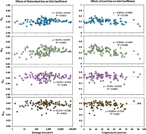
Figure 4. Gini Coefficients for discharge (Q), total nitrogen (TN), total phosphorus (TP), and total suspended sediment (TSS) as a function of drainage area and percentage of the watershed that is agricultural land use.
Download figure:
Standard image High-resolution imageZhang et al (2015) reported that major tributaries to Chesapeake Bay showed little temporal variability in their fractional contributions of TN, which was not the case for TP and TSS. This implies roughly similar long-term spatial patterns among these tributaries in terms of both N input and transport processes that convert variable climatic- and anthropogenic- driven input signals into comparatively persistent output signals at the edge of streams (Basu et al 2010, Guan et al 2011, Gall et al 2013). Specifically, TN is dominated by dissolved N, which is modulated by processes of subsurface transport, storage, and mixing that are relatively homogeneous over a range of spatial and temporal scales (Gall et al 2013, Kirchner and Neal 2013, Harman 2015). By contrast, particulate species are dominated by surface transport that are more susceptible to episodic exports (Zhang et al 2016).
3.2. Implications for temporal targeting
As the Gini Coefficient increases, the percentage of time over which a specific load is discharged decreases (figure 5). For example, at the NTN site with the lowest GTN value (Station ID #01493112, GTN = 0.25), 25% of the TN load exported during the study period occurred during 16% of the time. In contrast, at the site with the highest GTN value (Station ID #01610155, GTN = 0.73), 25% of the TN load was exported within sim 2% of the time (figure 5). The least percentage during which TP and TSS were exported was even smaller, with 25% of the TP and TSS loads exported in as little as 11% and 0.6% of the study period (Station ID #01614000, GTP = 0.94, GTSS = 0.98), respectively.

Figure 5. (a) 'Windows of Opportunity' for attaining desired load reduction goals for the range of Gini Coefficients observed across the Chesapeake Bay Watershed, with examples shown in green, yellow, and red for 25%, 50% and 75% load reduction, respectively, when G = 0.20 and (b) Inverse relationships between Gini Coefficient and the 'Window of Opportunity' to achieve 25% (circles), 50% (triangles), and 75% (squares) load reduction.
Download figure:
Standard image High-resolution imageOne implication of high temporal inequality is that to achieve a specific load reduction goal, a small 'window of opportunity' exists to effectively treat the constituents of interest. In the context of the Chesapeake Bay TMDL, a sub-basin needing to reduce the loads of TN, TP, and TSS by 40%, for example, will have a much more difficult time achieving that load reduction goal if each Gini coefficient (i.e. each temporal inequality of the flux) is high. Reduction measures would unrealistically need to effectively capture and treat every single event larger than the high flow target. The greater the temporal inequality of the loads, the more important it is to prioritize treatment of high flow over low flow events to achieve the targeted load reduction. Sub-basins with lower temporal inequality would theoretically be able to reach load reduction goals by treating a larger number of lower flow events, with more forgiveness in design since each event contributes a smaller percentage of the overall goal than is the case in sub-basins with high temporal inequality.
3.3. Decision-making framework
The results of the temporal inequality analysis were used to develop two example decision-making tables for the sub-basins with the low and high temporal inequality of nutrient and sediment loads (tables 2 and 3). These tables show the 'windows of opportunity' for effectively treating the exported loads. The major difference in targeting low versus high flow events to achieve a desired load reduction goal is the period of time over which the BMP must be effective for reducing loads. If low-flow events are targeted, then the period of time over which the BMP must be effective can be quite high. For Gaging Station ID #01618100 (GTN = 0.25, GTP = 0.37, and GTSS = 0.61), achieving a 20% load reduction of TN would require effectively treating low flows during 34.2% of the time or high flows during 9.4% of the time, while achieving 20% load reduction of TSS would require effectively treating low flows during 64.5% of the time or high flows during 1.7% of the time (table 2). The 'window of opportunity' for achieving the same load reduction of TN and TSS at Gaging Station ID # 01502500 (GTN = 0.54, GTP = 0.79, and GTSS = 0.88) is 56.9% if low flows were targeted or 2.9% if high flows were targeted for TN and 92.4% and 0.06% if low and high flows were targeted for TSS.
Table 2. Decision-making tables for temporal targeting total nitrogen (TN), total phosphorus (TP), and total suspended sediment (TSS) load reduction at USGS Gaging Station ID # 01618100, with relatively low temporal inequality (GTN = 0.25, GTP = 0.37, and GTSS = 0.61), by targeting either low-flow or high-flow conditions.
| TN load reduction goal | % of time (low flow) | Target low flow ( m3 s−1) | % of time (high flow) | Target high flow ( m3 s−1) | TP load reduction goal | % of time (low flow) | Target low flow ( m3 s−1) | % of time (high flow) | Target high flow ( m3 s−1) | TSS load reduction goal | % of time (low flow) | Target low flow ( m3 s−1) | % of time (high flow) | Target high flow ( m3 s−1) |
|---|---|---|---|---|---|---|---|---|---|---|---|---|---|---|
| 10% | 19.2% | <0.187 | 4.0% | >0.782 | 10% | 23.8% | <0.200 | 1.8% | >0.940 | 10% | 48.4% | <0.275 | 0.5% | >1.25 |
| 20% | 34.2% | <0.227 | 9.4% | >0.603 | 20% | 41.3% | <0.252 | 5.1% | >0.728 | 20% | 64.5% | <0.340 | 1.7% | >0.949 |
| 30% | 47.1% | <0.270 | 16.0% | >0.464 | 30% | 55.7% | <0.303 | 9.6% | >0.600 | 30% | 75.0% | <0.411 | 3.8% | >0.790 |
| 40% | 58.1% | <0.311 | 23.4% | >0.419 | 40% | 67.4% | <0.357 | 15.5% | >0.467 | 40% | 82.6% | <0.456 | 7.3% | >0.657 |
| 50% | 68.0% | <0.360 | 32.0% | >0.360 | 50% | 76.7% | <0.422 | 23.3% | >0.422 | 50% | 88.2% | <0.538 | 11.8% | >0.538 |
| 60% | 76.6% | <0.419 | 41.9% | >0.311 | 60% | 84.5% | <0.467 | 32.6% | >0.357 | 60% | 92.7% | <0.657 | 17.4% | >0.456 |
| 70% | 84.0% | <0.464 | 52.9% | >0.270 | 70% | 90.4% | <0.600 | 44.3% | >0.303 | 70% | 96.2% | <0.790 | 25.0% | >0.411 |
| 80% | 90.6% | <0.603 | 65.8% | >0.227 | 80% | 94.9% | <0.728 | 58.7% | >0.252 | 80% | 98.3% | <0.949 | 35.5% | >0.340 |
| 90% | 96.0% | <0.782 | 80.8% | >0.187 | 90% | 98.2% | <0.940 | 76.2% | >0.200 | 90% | 99.5% | <1.25 | 51.6% | >0.275 |
Table 3. Decision-making tables for temporal targeting total nitrogen (TN), total phosphorus (TP), and total suspended sediment (TSS) load reduction at USGS Gaging Station ID #01502500, with relatively high temporal inequality (GTN = 0.54, GTP = 0.79, and GTSS = 0.88), by targeting either low-flow or high-flow conditions.
| TN load reduction goal | % of time (low flow) | Target low flow ( m3 s−1) | % of time (high flow) | Target high flow ( m3 s−1) | TP load reduction goal | % of time (low flow) | Target low flow ( m3 s−1) | % of time (high flow) | Target high flow ( m3 s−1) | TSS load reduction goal | % of time (low flow) | Target low flow ( m3 s−1) | % of time (high flow) | Target high flow ( m3 s−1) |
|---|---|---|---|---|---|---|---|---|---|---|---|---|---|---|
| 10% | 40.9% | <14.9 | 1.0% | >168.8 | 10% | 67.5% | <27.8 | 0.04% | >389.7 | 10% | 83.3% | <43.3 | 0.04% | >514.0 |
| 20% | 56.9% | <22.0 | 2.9% | >111.9 | 20% | 83.6% | <44.2 | 0.2% | >241.5 | 20% | 92.4% | <66.7 | 0.06% | >293.8 |
| 30% | 68.6% | <28.3 | 5.8% | >79.3 | 30% | 91.1% | <62.0 | 0.7% | >189.2 | 30% | 95.9% | <95.4 | 0.3% | >231.6 |
| 40% | 77.5% | <36.5 | 9.9% | >58.6 | 40% | 95.0% | <85.8 | 1.4% | >144.4 | 40% | 97.7% | <123.7 | 0.7% | >185.5 |
| 50% | 84.6% | <46.2 | 15.4% | >46.2 | 50% | 97.3% | <114.4 | 2.7% | >114.4 | 50% | 98.7% | <147.5 | 1.3% | >147.5 |
| 60% | 90.1% | <58.6 | 22.5% | >36.5 | 60% | 98.6% | <144.4 | 5.0% | >85.8 | 60% | 99.3% | <185.5 | 2.3% | >123.7 |
| 70% | 94.2% | <79.3 | 31.4% | >28.3 | 70% | 99.3% | <189.2 | 8.9% | >62.0 | 70% | 99.7% | <231.6 | 4.1% | >95.4 |
| 80% | 97.1% | <111.9 | 43.1% | >22.0 | 80% | 99.8% | <241.5 | 16.4% | >44.2 | 80% | 99.9% | <293.8 | 7.6% | >66.7 |
| 90% | 99.0% | <168.8 | 59.1% | >14.9 | 90% | 99.9% | <387.9 | 32.5% | >27/8 | 90% | 100.0% | <514.0 | 16.7% | >43.3 |
3.4. Hot moments in hot spots
Overall, the relative importance of targeting hot moments in hot spots (relative to other locations in the watershed) varies by constituent, with TN generally exhibiting decreasing temporal inequality with increasing area-normalized loads, while TSS exhibited a generally increasing degree of temporal inequality with increasing area-normalized loads (figure 6). In contrast, GTP showed no trend with area-normalized loads of TP across the Bay watershed (figure 6). These results suggest that to best achieve load reduction goals in TN hot spots, low-flow targeting to treat TN transported during base-flow conditions is likely to be more effective, due to the likely impacts of legacy sources and long groundwater travel times to the sub-watershed outlets (i.e. the gaging station locations). For TSS, however, watersheds with the highest area-normalized loads also had the highest Gini Coefficients, implying that temporal targeting in TSS hot spots is even more important for achieving a specific load reduction goal than in an area with lower TSS loads. The lack of relationship between GTP and area-normalized loads suggests that targeting high-flow events to achieve load reduction goals is relatively equally necessary across the entire watershed, with little difference between areas considered to be 'hot spots' and areas with lower loads.

Figure 6. Gini Coefficients for (a) total nitrogen (GTN); (b) total phosphorus (GTP); and (c) total suspended sediment (GTSS) as a function of area-normalized loads, for 108 USGS gaging stations across the Chesapeake Bay Watershed.
Download figure:
Standard image High-resolution image
Consequently, selection and location of BMPs in a sub-basin needs to consider both the spatial and temporal inequalities of the sub-basin. For example, one of the most common structural BMPs, riparian buffers, is known to have lower effectiveness during higher flow events (Gall et al 2018; Liu et al 2017), but is most effective when spatially located to intersect shallow sheet flow (Piechnik et al 2012, Wallace et al 2018). Other BMPs to effectively capture high flow events may need to capture and treat the runoff over extended periods of times, such as retention ponds or detention basins, that are common in urban/suburban settings but less commonly implemented in agricultural landscapes. Such technologies would reduce the temporal inequality of the flow and loads by reducing the peaks and releasing them over an extended duration of time. Additionally, adopting BMPs that are spatially located, such as cover crops and no-till practices, that collectively work to control sediment and nutrient loss may help to reduce the temporal inequality of the sub-basin by minimizing their occurrence and reducing 'first flush' effects.
4. Conclusion
The overall goal of this research was to quantify the temporal inequality of TN, TP, and TSS at 108 gaging stations in the Chesapeake Bay Watershed. Lorenz Curves and Gini Coefficients were calculated for an 8 year study period (water years 2010–2018). The results were used to develop a decision-making tool that could allow decision makers to more strategically identify the 'windows of opportunity' to target to best achieve a specific load reduction goal. Sites with higher temporal inequality have the potential to achieve load reduction goals during a relatively small portion of time if high-flow events are targeted. If only low-flow events are treated effectively, the results of the temporal inequality analysis suggest that some load reduction goals may not be possible unless BMPs are designed to also treat high-flow events.
This framework emphasizes the importance of temporal targeting 'windows of opportunity' during either low-flow (i.e. baseflow conditions) or high-flow (i.e. large storm) events, with low-flow events being relatively more important for TN compared to TP and TSS. Overall, the approach provides a uniform method for quantifying temporal inequality and targeting 'hot moments' in 'hot spots' to best achieve load reduction goals in impaired watersheds.
Acknowledgments
Heather E. Preisendanz (Gall) is funded, in part, by the Penn State Institutes of Energy and the Environment and by the USDA National Institute of Food and Agriculture Federal Appropriations under Project PEN04574 and Accession number 1 004 448. Qian Zhang is funded by the Environmental Protection Agency/Chesapeake Bay Program Technical Support Grant No. 07-5-230 480. All entities involved are equal opportunity providers and employers. Heather E. Preisendanz would like to acknowledge her daughter, Maya Gall, for her understanding and patience during the final writing stages of this publication, which occurred during the remote working environment during the COVID-19 pandemic that turned living rooms into home offices at the time this paper was completed and submitted.
Data availability statement
The data that support the findings of this study are openly available at the following URL/DOI: https://cbrim.er.usgs.gov.