

Abstract
The stratospheric influence on summertime high surface ozone ( ) events is examined using a twenty-year simulation from the Whole Atmosphere Community Climate Model. We find that
  transported from the stratosphere makes a significant contribution to the surface
  variability where background surface
  exceeds the 95th percentile, especially over western U.S. Maximum covariance analysis is applied to
  anomalies paired with stratospheric
  tracer anomalies to identify the stratospheric intrusion and the underlying dynamical mechanism. The first leading mode corresponds to deep stratospheric intrusions in the western and northern tier of the U.S., and intensified northeasterlies in the mid-to-lower troposphere along the west coast, which also facilitate the transport to the eastern Pacific Ocean. The second leading mode corresponds to deep intrusions over the Intermountain Regions. Both modes are associated with eastward propagating baroclinic systems, which are amplified near the end of the North Pacific storm tracks, leading to strong descents over the western U.S.
Export citation and abstract BibTeX RIS
1. Introduction
Surface ozone ( ) adversely affects human health and the ecosystem because of its high oxidation capability (U.S. Environmental Protection Agency, 2015). The risk of
  pollution on mortality is also significantly raised by high temperatures (Levy and Patz 2015). During summer, surface
  level maximizes over the western U.S. (Gaudel et al 2018), mainly attributed to the combination of active photochemical production and noncontrollable sources, such as intercontinental pollution transport, lightning, and wildfire events (Fiore et al 2002, Jaffe et al 2018). Downward transport of
  during stratospheric intrusions is also considered to be a contributing factor during summertime (Danielsen 1980, Lefohn et al 2011, Lefohn et al 2012, Zanis et al 2014, Akritidis et al 2016, Yang et al 2016, Škerlak et al 2019). The transport is achieved irreversibly by a tongue-like structure containing high stratospheric
  extruding downward, folding into the tropospheric air and descending toward the surface (Danielsen 1968, Johnson and Viezee 1981). When a stratospheric intrusion contributes high
  to the surface, in addition to that produced by anthropogenic pollution, it could easily push the surface
  values beyond the National Ambient Air Quality Standard threshold 70 ppbv (Langford et al 2017, Škerlak et al 2019). Observational and modeling studies have shown that surface
  extremes that are directly associated with downward transport from the stratosphere preferentially occur in the western U.S. (Stohl et al 2003, Lin et al 2012, Lin et al 2015, Škerlak et al 2014). Consequently, the joint effects of chemistry and episodic stratospheric transport make the western U.S. a hot spot of
  pollution in summer.
Due to the large dynamic variability of the tropopause, limited temporal and spatial extent of measurements, and mixing with tropospheric air, the observations of transport due to stratospheric intrusions are challenging (Stohl et al 2003). In addition, most of the previous studies focused on springtime stratospheric influence because tropopause  abundances and downward air mass fluxes maximize during that time (Langford 1999, Prather et al 2011, Langford et al 2009, Langford et al 2012, Lin et al 2012, Lin et al 2015, Langford et al 2017, Albers et al 2018). The linkage between summertime stratospheric intrusion and high surface
  events over the western U.S. has received less attention (Lefohn et al 2011, Lefohn et al 2012). By analyzing the output of a state-of-the-art chemistry climate model implemented with an artificial stratospheric ozone tracer (
 S), we aim to 1. estimate the contribution of
  reaching the surface associated with summertime stratospheric intrusions, 2. understand the space-time behavior of stratospheric intrusion events, and 3. clarify the underlying dynamical mechanism.
2. Methods
2.1. CESM2(WACCM6) and O3S Diagnostic
We analyzed daily surface  and stratospheric
  tracer (denoted by
  S) from 1995 to 2014 summer months (June–August, JJA) using the Whole Atmosphere Community Climate Model version 6 (WACCM6) of the Community Earth System Model version 2 (CESM2). It is the high-top version of the Community Atmosphere Model version 6 (CAM6), integrating the atmospheric physics and chemistry from the surface to nearly 140 km. The WACCM6 uses the same atmospheric physics as CAM6. The chemical mechanism includes comprehensive troposphere, stratosphere, mesosphere and lower thermosphere chemistry, described by Emmons et al (2020). The standard emissions are based on anthropogenic and biomass burning inventories specified for the Coupled Model Intercomparison Project 6 (CMIP6). WACCM6 is coupled to the interactive Community Land Model version 5 (CLM5), which handles dry deposition. The simulations shown here are fully coupled ocean-atmosphere experiment, and feature
  (latitude× longitude) horizontal resolution and 70 layers, with ∼1.2 km vertical resolution above the boundary layer to the lower stratosphere. We consider WACCM6 is well suited for studying the transport during stratospheric intrusion because that 1. the atmospheric chemistry and deposition scheme for
  are well represented and tropospheric
  simulations are improved in comparison to observations (Emmons et al 2020); 2. WACCM6 is able to effectively reproduce the observed wind and temperature climatologies as well as stratospheric variability (Gettelman et al 2019); 3. the twenty-year simulation with daily output of
  and
and  S provides us with large samples to study. Detailed model formulations, descriptions, and evaluations can be found in Gettelman et al (2019) and Emmons et al (2020).
To quantify the stratospheric contribution to high surface  events, we study an artificial tracer,
  S, for
  originating in the stratosphere, which is implemented in a manner as described in Tilmes et al (2016).
  S experiences the same loss rate as
  in the troposphere but is not affected by
  photolysis as defined by the Chemistry-Climate Model Initiative (CCMI). Earlier studies have shown that the diagnostics of deep stratospheric intrusions are insensitive to the choice of tropopause definition (Yang et al 2016) or
  S tagging methods (Lin et al 2012).
2.2. Maximum covariance analysis
Maximum Covariance Analysis (MCA), known as Singular Value Decomposition (SVD) analysis, is a useful tool for detecting coherent patterns between two different geophysical fields (e.g. (Bretherton et al 1992, Hurrell 1995, Dai 2013)). In this study, we isolate pairs of spatial patterns and corresponding time series by performing the eigenanalysis on the temporal covariance matrix between  anomalies and
  S anomalies at the lowest model level (detailed calculations are discussed in (Bretherton 2015)). Daily anomalies of
  and
and  S at the lowest model level are derived with respect to the twenty-year (1995–2014) mean of that day. The considered domain in this study is 20°–50°N, 70°–140°W.
3. Results
3.1. Evaluation of CESM2 (WACCM6)
Here we first evaluate the WACCM6 simulations against observations from the Tropospheric Ozo-ne Assessment Report (TOAR) (Schultz et al 2017). Figure 1(a) is the 1995–2014 mean of 'all$mean' variables from the TOAR  (latitude× longitude) monthly median products. High
  values (
 ) are seen over the western U.S. in TOAR measurements. For WACCM6, we have gridded the simulations onto the horizontal grid of TOAR data and calculated median
  concentrations using the same metrics to guarantee an apple-to-apple comparison (see figure 1(b). Generally a good agreement is found between the model and observations over the Central U.S. and most of the West Region, with percentage differences within 15% (see figure S1 (https://stacks.iop.org/ERL/15/1040a6/mmedia)). However, WACCM6 overestimates the surface median
  over the southeast U.S. by 55% (
 ), which is consistent with the evaluation in Emmons et al (2020). The biased O3 over the eastern U.S. is a long existing problem that can have various reasons starting with still insufficient complexity of the chemistry, but also the model resolution, deposition scheme, etc (Schwantes et al 2020).
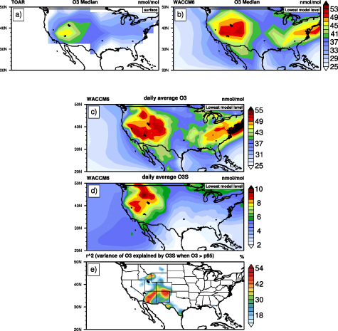
Figure 1. Twenty-year (1995–2014) mean of summertime surface  median values (a) observed from the TOAR and (b) simulated in WACCM6 at the lowest model level with 5° latitude × 5° longitude resolution. (c, d) Mean of daily average
  and
and  S simulations at the lowest model level in the same time period, respectively. Note the ranges of color bars are different. (e) R2 in color shows the near-surface
  variance explained by surface
  S when surface
 95th percentile at each grid cell during 1995–2014 summer.
Download figure:
Standard image High-resolution imageFigure 1(c) and (d) shows the 1995–2014 mean of daily  and
and  S simulations in
  (latitude× longitude) resolution at the lowest model level, respectively. Figure 1(c) is similar to figure 1(b) and shows that high
  are concentrated over the western U.S. As shown in 1(d), strong stratospheric impact, ranging from 6 to 10 nmol/mol, is found over the Canada-U.S. border and the Western States, including southern British Columbia, Washington, Oregon, Idaho, Montana, Wyoming, California, Nevada, Utah, Arizona, and Colorado. Our model simulation is in agreement with previous observational studies which reported that deep stratospheric intrusions preferentially occur in the West and the Intermountain West (Brioude et al 2007, Bourqui and Trépanier 2010, Ambrose et al 2011, Lefohn et al 2011, Lefohn et al 2012, Lin et al 2012, Langford et al 2012, Langford et al 2015, Langford et al 2017, Clark and Chiao 2019). A minimum stratospheric impact occurs in the Southeast, in good agreement with results in Lin et al (2012). These features are also consistent with simulations by the Geophysical Fluid Dynamics Laboratory global chemistry-climate model (Clifton et al 2014). Additionally, the simulated stratospheric impact in late spring (figure S2) agrees well with that shown in figure 11(c) and (d) from Lin et al (2012).
We now estimate the importance of  S on surface
  . We calculate the percentage of variance (r2) of surface
  explained by surface
  S when surface
  exceeds the 95th percentile (p95, hereinafter) value at each grid point during 1995–2014 summer months using daily average
  and
and  S (see figure 1(c) and (d)). The linear trend has been removed before the calculation. As suggested in figure 1(e), high peaks are located over Wyoming, southern Texas, and the Four Corners area (Colorado, Utah, Arizona, and New Mexico). We see in Arizona, for example,
  S can explain as high as 54% of surface
  variance during days in which surface
  exceeds p95. We compare our results with those from prior observational studies. Lefohn et al (2012) studied stratospheric intrusion events associated with daily maximum hourly
  in exceedance of
  at both rural and urban monitoring sites of the U.S. Statistically significant relations are found over the southern Texas, Arizona, Colorado, Utah, Nevada, California, and Wyoming in summer months during 2006–2008. Overall, our model simulations support observational findings that stratospheric intrusions coincident with
  preferentially take place in the West and Intermountain West during summertime. We also quantify the stratospheric impact when surface O3 exceeds p95 at each grid cell and find that in regional average over the western U.S. (
 N, 100°W–125°W), the stratospheric contribution is 18.4% (not shown).
3.2. MCA results and interpretation
We employ MCA to investigate how surface  is related to
  S reaching the surface on daily basis. The first two leading modes are summarized in figure 2. Together, these two modes explain 60% of the covariance pattern over the domain of interest. The first mode shows large positive covariances over the eastern Pacific, western and northern tier of the U.S. (figure 2(a). The second mode shows dipole structure with
  and
and  S surplus over the western U.S. and deficit over the east (figure 2(b). Surface level
  S anomalies are found to lag the 200–500 hPa
  S anomalies by two days (not shown), suggesting the downward influence. No significant lead-lag relationships are found either between the expansion coefficient time series (loadings) of
  and
and  S at the surface or between the first two SVD modes.

Figure 2. Spatial and temporal patterns of the two leading modes from MCA with (a) Mode 1 on the left and (b) Mode 2 on the right. Upper panels show the covariance patterns between surface  anomalies and surface
  S anomalies on daily bases in JJA over 1995–2014. Red (blue) color shadings represent positive (negative) values. The number shown in the top center is the portion of the covariance explained by each mode. Below are the standardized anomalies of the loadings with red lines representing the principal component coefficients of surface
  anomalies in summer from 1995 to 2014 and blue for surface
  S anomalies. Black circles indicate the occurrences of the high surface
  events as defined in the text.
Download figure:
Standard image High-resolution imageWe identify ∼20 days per month (1404 days in twenty years for the first two leading modes) when both expansion coefficient time series are greater than 0, indicating that surface O3 concentration increase is coincident with O3S reaching the surface. Lefohn et al Lefohn et al (2011), Lefohn et al (2012) investigated the frequency of surface O3 enhancements that are associated with stratosphere-to-troposphere transport down to the surface across the U.S. and reported that the average number of days per month ranges from 16 days to 23 days at monitoring sites in the West and Intermountain West in summer months. Our results of intrusion frequency are in remarkable agreement with their results.
Next, we define high surface O3 events caused by stratospheric intrusions when both loadings exceed 1.5 standard deviations, as marked by black circles in figure 2. Each event lasts for a few days. Based on this definition, composite analyses according to high surface  events are carried out using
  S daily data. The composited patterns are not sensitive to the thresholds we chose for the analyses. Schematics in figure 3 show the large amplitude composited
  S structures and near-surface circulations corresponding to both modes. We use neon yellow color to highlight the area with
  S larger than
  , which can be treated approximately as the tropopause (Yang et al 2016). During Mode 1, depressed tropopause height followed by enhanced
  S can be found around 50°N, 120°W (figure 3(a). Since stratospheric air contains higher values of potential vorticity (PV) and
  , the intrusion of the tropopause tends to replace the tropospheric air by ozone-rich stratospheric air with large PV (Danielsen 1968, Mote et al 1991, Wimmers et al 2003). Transport of
  S to low levels is tied to stratospheric intrusions and strong subsidence in the troposphere. Figure 4(d) shows a map of composited means of 500 hPa vertical velocity (ω) anomalies on the day of the events corresponding to Mode 1. The intrusion is associated with intensified subsidence on the U.S.-Canada border. Coherently, enhanced
  S on the northern tier can be seen throughout the troposphere, while the maximum over the Pacific appears below 700 hPa (figure 3(a)). We conduct composited analyses on anomalies of 860 hPa geopotential height as well as surface winds according to events of Mode 1. A quadrupole pattern of low-level geopotential height anomalies is seen over the North American continent. In contrast to the positive correlation between the upper-level cyclonic vorticity and
  S (figure S3a), low-level geopotential height and
  S reaching the surface are strongly anti-correlated (figure 3(b)). Dry air (figure S3b) with high PV value (figure S3a) descends on the northern tier of the U.S. as a result of stratosphere-to-troposphere transport by intensified subsidence. Warm and moist tropospheric air is seen (figure S3b–c) downstream (east) of the surface low. In addition to the anomalous descent, we also see a strengthening of northeasterly along the west coast near the surface (figure 3(b)). This intensified easterly associated with stronger anticyclone facilitates the horizontal transport towards the subtropical Pacific in the mid-to-lower troposphere (figure 3(a)).

Figure 3. (a) Composited  S structure of high surface
  events for Mode 1. For illustrative purpose, scatter plot includes only the grid points with
  S
S 
 . (b) A map of 860 hPa geopotential height anomalies (in color, unit is m) and surface wind anomalies (in vectors, m s−1) composited to the defined high surface
  events for Mode 1. The hatching denotes that the geopotential height anomalies are not statistically significant at the 95% confidence level using the Student's t test. (c) (d) are similar to (a) (b) but for Mode 2. For illustrative purpose, scatter plot (c) includes only the grid points with
  S
S 
 .
.
Download figure:
Standard image High-resolution image
Figure 4. Snapshots of composited mean of 500 hPa ω anomalies (in colors, Pa/s) and 200 hPa zonal winds (in contours, m s−1) when large events occur for Mode 1 (left) and for Mode 2 (right) during (a, e) day −6, (b, f) day −4, (c, g) day −2, (d, h) day 0. Red (blue) colors indicate regions with anomalous descent (ascent). Contour interval is 3 m s−1. Stippling indicates that the ω anomalies are statistically significant at the 95% confidence level using the Student's t test. The navy dashed line marks the location of 200 hPa jet axis.
Download figure:
Standard image High-resolution imageDuring Mode 2 (figure 3(c)), the intrusion occurs around 40°N, 115°W. Surface  S maximum is concentrated over the Intermountain West, such as Colorado, Arizona, Utah, Nevada. Different from Mode 1, a dipole pattern of the low-level geopotential height anomalies is seen over the continental U.S. Large values of negative geopotential height anomalies are observed above the intermountain regions (figure 3(d) aligned with cold dry air and positive PV anomalies (figure S4a–c) subsiding west of the surface low pressure while rising warm and moist air occur on the east (figure 4(h) and figure S4b–c).
During both modes, the  S reaching the surface can be 10–
 (see surface contours of figure 3(a) and 3(c), respectively). In regional average over the western U.S. (30°N–50°N, 100°W–125°W, the stratospheric contribution is 11 nmol/mol. The amplitude agrees well with the observational record from the California Baseline Ozone Transport Study (CABOTS), in which they found that stratospheric contribution is 10–
 to the surface over Northern California during an intrusion case in August 2016 (Clark and Chiao 2019). We also see ∼10 days per summer season when high surface O3 events associated with the first two SVD modes occur, with variation across years.
3.3. Dynamical mechanism
Next we examine the dynamical mechanism underlying the stratospheric intrusion events associated with Mode 1 and Mode 2. Figure 4 shows the time evolution of 500 hPa vertical velocity (ω) anomalies and 200 hPa zonal winds for the composites based on high  and
and  S events in Mode 1 (figures 4(a)–(d) and Mode 2 (figure 4(e)–(h), respectively. The positions of the upper-level jet axis are marked by dashed lines. The downstream development (Chang 1993), characterized by eastward propagation of the wave systems, can be seen in both modes.
More specifically, for Mode 1, the large descending anomaly is centered at 50°N, 160°W on day −6 (figure 4(a). After 2 days, it shifts eastward following the continuous jet (figure 4(b). On day −2, the descending center manifests near the west coast (figure 4(c), consistent with the result that relationship of 500 hPa  S with the principal component of Mode 1 is maximized about two days ahead of surface
  S peaks (not shown). During day −2 to day 0, the subsidence stays close to the U.S.–Canada border, embedded within the jet stream (figure 4(d). On day 0, the strong descent on the northern tier of the U.S. continuously facilitates the downward transport of
  S toward the surface (figure 3(a).
Regarding Mode 2, large disturbance center can be seen on day −6 near the eastern Pacific (figure 4(e)). From day −4 to day −2, the descending center continues to grow near 135°W (figure 4(f)–(g)). The downstream side strengthens remarkably near 125°W where the jet breaks. On day −2, strong anomalous subsidence reaches the western U.S. whereas ascending anomalies are triggered on the east. It is the enhanced subsidence that induces the stratospheric intrusion and downward transport of stratospheric  (figures 4(h) and 3(c)).
During boreal summer, the dominant upper-level circulation consists of westerly jet north of 40°N, together with frequent eastward traveling baroclinic waves (White 1982). The baroclinic waves commonly exhibit life cycles of baroclinic growth and barotropic decay along the storm track regions (Simmons and Hoskins 1978, Blackmon et al 1984). Observational and modeling studies have revealed that the baroclinic disturbances leave imprint on atmospheric composition. Aircraft experiments provided evidence that high amounts of stratospheric radioactive debris and ozone were drawn into the troposphere by midlatitude storms (Danielsen 1968). Schoeberl and Krueger (1983) and Mote et al Mote et al (1991) identified the coherent fluctuations in total  and medium scale waves along the wintertime oceanic storm track regions using satellite data. Stone et al (1996) found baroclinic wave features using upper tropospheric water vapor measurement. General circulation model was capable of representing stratosphere–troposphere exchange associated with baroclinic waves in midlatitudes (Mote et al 1994). In our study, baroclinic wave system and its resulting circulation is also found important for the occurrence of deep stratospheric intrusions over the western U.S. in summertime (Sprenger and Wernli 2003).
In both modes, we see that the wave trains originate over the baroclinically unstable central Pacific, grow by baroclinic conversion, radiate energy downstream through ageostrophic geopotential fluxes, and dissipate over the jet exit near the western U.S., as discussed in previous studies (Chang and Orlanski 1993, Chang 1993). The upper-level jet stream acts as a wave guide, constraining the baroclinic system tightly along its core. From day −2 to day 0 in both modes, the intensified descents at 500 hPa, which corresponded to the downward transport of  S, are evident near the western U.S. (115°–120°W). These two modes mainly differ by the location of the jet core. For Mode 1, the jet is almost continuous across the North Pacific and the averaged jet axis is located at 46°N. The passage of the wave trains takes about 8 days, starting from central North Pacific (40°N, 170°W, see figure 5(a), propagating eastward to the U.S.–Canada border (45°N, 120°W). For Mode 2, the polar jet and the subtropical jet are well separated. The successive baroclinic waves develop rapidly, beginning with a large descending anomaly at the jet exit (40°N, 140°E) from day −6, ending with a trough on the west-and-a ridge on the east over the continental U.S. (figure 3(d)).
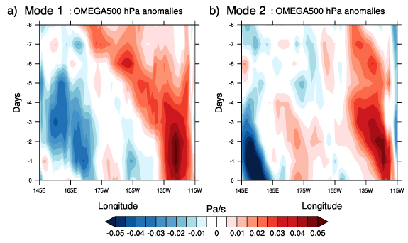
Figure 5. Days versus longitude diagrams of ω anomalies (Pa/s) at 500 hPa (a) along the band of 200 hPa jet axis for Mode 1 and (b) along 38°N for Mode 2, respectively.
Download figure:
Standard image High-resolution image
Finally, Hovmöller diagrams are constructed to summarize the eastward propagating baroclinic systems that occur prior to high surface  and
and  S events. The longitude-time plots of 500 hPa ω anomalies along the latitudinal band of the jet axis are depicted for both modes (figure 5). More specifically, figure 5(a) is the ω anomalies along the jet axis as marked in figure 4(a)–(d) while figure 5(b) is plotted along 38°N for simplicity. We can see a sequence of downstream developing wave train originating from the North Pacific and propagating along the upper-level jet. Eastward propagation of Mode 2 is less clear than that of Mode 1. The descending anomalies begin to amplify near the jet exit two days before the deep intrusions over the western U.S. Similar conclusions are also found using upper-level meridional velocity (not shown). The results are consistent with evolving of baroclinic waves, and are in good agreement with the wave train signature diagnosed in Lim and Wallace (1991) and Chang (1993), in terms of their structure, magnitude, and traveling speed. To sum up, the large
  events caused by deep intrusions are associated with eastward propagating baroclinic systems tied closely to the North Pacific storm tracks, with enhanced wave amplitudes and descents over the jet exit region near the western U.S.
4. Conclusions and discussions
Our study has examined high surface  events associated with downward transport from the stratosphere over the U.S. during summertime, when high temperature could further increase the impact of
  pollution on mortality. By analyzing a twenty-year (1995-2014) simulation by CESM2 (WACCM6), we have found that the stratospheric O3 can explain as high as 54% of surface O3 variability when surface
  exceeds 95th percentile, and the regional averaged stratospheric contribution is ∼18% over the western U.S. We have further analyzed the circumstances when stratospheric intrusions of ozone covary with surface
  anomalies over the region of 20°–50°N and 70°–140°W on daily basis using MCA. The first two leading modes explain 60% of the total covariance pattern. In Mode 1, deep stratospheric intrusions occur preferentially over the northwestern U.S. The associated intensified northeasterly wind anomalies over the west coast further brings continental
  S towards the Pacific Ocean. In Mode 2, deep stratospheric intrusions occur over the Intermountain West. The composited O3S values reaching the surface associated with these two SVD modes range from 10 to 18 nmol/mol. In regional average over the western U.S., the stratospheric contribution is 11 nmol/mol. Both modes are results of eastward propagating wave trains, originating from the central North Pacific and amplifying near the jet exit, with enhanced subsidence over the western U.S.
We have also repeated our MCA analysis to demonstrate the robustness of the dynamical mechanism across seasons. The first leading mode and corresponding anomalous ω evolution prior to intrusion events for winter, spring, and fall seasons are summarized in figures S5–7. The first leading modes during each of the seasons explain ∼40% of covariance between  and
and  S. Similarly, we find that the strongest disturbance extends from the central North Pacific to the west coast of the U.S. during day −6 to day −4. During day −2 to day 0, the descents strengthen remarkably over the west coast while new ascending centers develop on the downstream side. The downward
  transport is typically regulated by upper-level jet streams across seasons, consistent with previous studies (Langford 1999, Lin et al 2015, Albers et al 2018).
Overall, our study has demonstrated that summertime stratospheric intrusions, though infrequent, can contribute crucially to surface  extremes over the Western U.S. These stratospheric intrusion events are caused by strong subsidence in the region, which is a result of eastward propagating baroclinic waves originating from the central North Pacific Ocean. However, a few caveats have to be noted. WACCM6 overestimates tropospheric
  and thus the exact contribution of stratospheric intrusion to surface should be treated with caution. Additionally, our diagnostic is based on one single climate model because of the use of daily
  S output. It's worth performing similar analyses in other chemistry climate models to assess the robustness of the conclusions. Future work will also be devoted to 1. studying simulations with high spatiotemporal resolution at certain hot spot areas so that our results can directly benefit air pollution management, and 2. understanding the origination of upstream baroclinic disturbance so that we can improve the predictability of such
  extremes associated with summertime stratospheric intrusions.
Acknowledgments
We thank Drs Sasha Glanville, Gang Chen, Olivia Clifton, Xiaomeng Jin, Arlene Fiore, Mingfang Ting, Douglas Kinnison, and Ben Li for helpful discussion. We are grateful to Drs Dimitris Akritidis and Tom Ratkus for constructive suggestions in data visualization. We thank four anonymous reviewers for their valuable comments, which helped to greatly improve the manuscript. The CESM project is supported primarily by the National Science Foundation (NSF). Computing and data storage resources, including the Cheyenne supercomputer (doi:10.5065/D6RX99HX), were provided by the Computational and Information Systems Laboratory at NCAR. XW and YW are supported by NSF Award AGS-1802248. XW also acknowledges the support from NCAR's Advanced Study Program's Graduate Visitor Program and PCCRC.
Data Availability Statement
The data that support the findings of this study are available upon request from the authors. All WACCM6 simulations were carried out on the Cheyenne high-performance computing platform (https://www2.cisl.ucar.edu/user-support/acknowled-ging-ncarcisl), and are available at NCAR's Campaign Storage upon acceptance.