

Abstract
Air pollutants seriously impact climate change and human health. In this study, the gridpoint statistical interpolation (GSI) three-dimensional variational data assimilation system was extended from ground data to vertical profile data, which reduced the simulation error of the model in the vertical layer. The coupled GSI-Lidar-WRF-Chem system was used to improve the accuracy of fine particulate matter (PM2.5) simulation during a wintertime heavy pollution event in the North China Plain in late November 2017. In this experiment, two vehicle-mounted Lidar instruments were utilized to make synchronous observations around the 6th Ring Road of Beijing, and five ground-based Lidars were used for long-term network observations on the North China Plain. Data assimilation was then performed using the PM2.5 vertical profile retrieved from the seven Lidars. Compared with the model results, the correlation of assimilation increased from 0.74–0.86, and the root-mean-square error decreased by 36.6%. Meanwhile, the transport flux and transport flux intensity of the PM2.5 were analyzed, which revealed that the PM2.5 around the 6th Ring Road of Beijing was mainly concentrated below 1.8 km, and there were obvious double layers of particles. Particulates in the southwest were mainly input, while those in the northeast were mainly output. Both the input and output heights were around 1 km, although the input intensity was higher than the output intensity. The GSI-Lidar-WRF-Chem system has great potential for air quality simulation and forecasting.
Export citation and abstract BibTeX RIS

Original content from this work may be used under the terms of the Creative Commons Attribution 4.0 license. Any further distribution of this work must maintain attribution to the author(s) and the title of the work, journal citation and DOI.
1. Introduction
As the most populous country in the world, China is facing serious challenges from the environmental pollution associated with the rapid industrial development in recent years (Qiang et al 2011). Fine particulate matter (PM2.5) is the most prominent pollutant in China, which ranks among the most polluted countries in the world (Zhang and Cao 2015, Lv et al 2017a). Meanwhile, PM2.5 exerts serious impacts on sustainable urban development, the ecological environment, and human health (Carmichael et al 2009, Michiels et al 2012, Silva 2015). Studies have shown that PM2.5 pollution contributes to more than 1 million premature deaths in China each year (Zhang et al 2017, Wang et al 2017, Ren et al 2017) and originates primarily from local emissions and regional transport (Subramanian et al 2007, Ck et al 2010, Udduttula 2014, Ho et al 2015). Therefore, providing an accurate three-dimensional distribution of PM2.5 is particularly important for the analysis of PM2.5 sources and for the government departments that specify emission reduction decisions (Zhang et al 2015, Gao et al 2015, Sun et al 2016).
Observations and air quality models are the key methods used to obtain the regional distribution characteristics of PM2.5. Lidar can capture the vertical distribution of PM2.5 in situ (Ortiz-Amezcua et al 2017, Osborne et al 2019, Foth et al 2019), while the regional distribution of PM2.5 requires help from the WRF-Chem, CMAQ, and other air quality models (Campbell et al, 2017, Cuchiara et al 2017, Bran and Srivastava 2017, Podrascanin 2019). These air quality models include large uncertainties in their PM2.5 simulation results, however, with the errors mainly originating from emission inventory, meteorological conditions, and various model assumptions (Tsao et al 2012, Crippa et al 2016, Li et al 2018). Meanwhile, the development in recent years of deep learning models, machine learning, and other dependent computer models has also resulted in improved performance (Vu et al 2019, Smith et al 2019), although since these models are black boxes independent of physical relationships, the impacts of input variables cannot be analyzed. Fortunately, data assimilation (DA) is a powerful technique for combining models and observations, which can be used to correct model simulation results, greatly increase simulation accuracy, and improve precision (Maxwell et al 2009, Zhang et al 2016, Ma et al 2018).
In recent years, however, the assimilation of particulate matter data has mainly focused on ground observation data (Jiang et al 2013, Gao 2015, Gao et al 2017, Robichaud 2017) and satellite remote sensing data (Liu et al 2011, Schwartz et al 2012, Saide et al 2013, 2014, 2015), while the DA of Lidar data has rarely been examined.
In this study, two vehicle-mounted Lidars were first used to make synchronous observations along the 6th Ring Road of Beijing, and five ground-based Lidars (Chen et al 2016, Xiang et al 2019) were employed for long-term network observations on the North China Plain. Second, a model for the conversion of the extinction coefficient to aerosol mass concentration was utilized to invert the vertical PM2.5 concentration. Third, the observed vertical PM2.5 and the simulated results obtained using WRF-Chem were coupled to the gridpoint statistical interpolation three-dimensional variational (GSI 3DVAR) DA system (Pagowski et al 2014), and PM2.5 data with high precision were obtained by correcting the measured data. Finally, the transport flux (TF) and the transport flux intensity (TFI) of the PM2.5 in the region were analyzed. In addition, pollution transport paths were evaluated using the backward trajectory model.
2. Materials and methods
2.1. Instrumentation
The overall structure of the Mie Lidar system consists of an emitting system, receiving system, data acquisition system, control system, and GPS system (Lv et al 2017b). The emitting system comprises a laser and an emission optical unit. The receiving system is designed based on the principle of the Cassegrain optical telescope, which has a 1-mard receiving field of view with a vertical resolution of 7.5 m. The data acquisition and control system comprise one of the key components used to determine the data quality of the Lidar. In addition, the response speed, bandwidth, dynamic range, and signal-to-noise ratio of the measured electronic system directly determine the spatial and temporal resolutions of the Lidar system and the analytical ability of weak signals. The main technical parameters of the Lidar system are listed in table S1 (available online at stacks.iop.org/ERL/15/094071/mmedia). Additional details regarding the ground-based Lidar information can be found in Xiang et al (2019).
2.2. Experimental
In this study, we established two vehicle-mounted Lidars and five ground-based Lidar networks, covering the Beijing-Tianjin-Hebei region. The two vehicle-mounted Lidars performed closed observations along the 6th Ring Road of Beijing at 1:40 p.m. local time on 27 November 2017. One vehicle started north of the 6th Ring Road and traveled clockwise to the starting point, while the other vehicle started south of the 6th Ring Road. The observation route of the 6th Ring Road in Beijing is depicted by the red curve in figure 1. The 6th Ring Road in Beijing is a circular expressway with four lanes in two directions and a total length of approximately 187.6 km. The vehicle speed was set to 70 km h−1 in order to maximize the detection precision, detection time, and other factors. The two vehicles returned to the starting position at 4:20 p.m. on the same day. Meanwhile, the blue stars in figure 1 represent the five ground-based Lidar networks, which were used for long-term continuous observations of the Beijing-Tianjin-Hebei region. The observation data from 26–29 November 2017, were selected to analyze the pollution status of the Beijing-Tianjin-Hebei region.
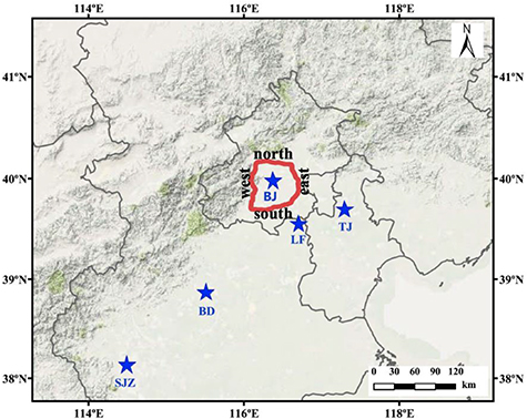
Figure 1. Locations of field observation sites. The red curve is the monitoring path of the vehicle-mounted Lidar. The blue stars represent the ground-based Lidar networks, BJ, LF, TJ, BDm and SJZ signify Beijing, Langfang, Tianjin, Baoding, and Shijiazhuang, respectively.
Download figure:
Standard image High-resolution image2.3. Retrieval method
2.3.1. Particle extinction coefficient
The Lidar equation for the retrieved aerosol Lidar signal can be written as
where  is the received aerosol Lidar signal at the height of z,
  is the wavelength of laser, K is the correction constant related to the Lidar system,
  is the power to launch a laser beam, A is the optical receiving area of the receiving telescope, and
  is the height of the Lidar system.
  and
and  are the aerosol backscatter coefficient and molecular backscatter coefficient, respectively.
  and
and  the aerosol extinction coefficient and molecular extinction coefficient, respectively.
Previous studies have shown that compared with the Collis method (Collis and Russell 1976) and the Klett method (Klett 1981), the Fernald method (Fernald 1984) was the most stable, mature, and accurate inversion method. Therefore, the extinction coefficient of aerosols was retrieved using the Fernald method. The Fernald method assumes that the scattering of particles is proportional to the extinction coefficient for both aerosols and molecules. As shown in the following equations (2) and (equation (3)), where  is the ratio of extinction coefficient and backscatter coefficient in atmospheric aerosol (usually also referred to as the Lidar ratio), which was set as 50 Sr in this study. Moreover,
  is the ratio of extinction coefficient and backscatter coefficient in atmospheric molecules, which was calculated as
  according to the atmospheric molecular model
Therefore, the equation (equation (1)) for the aerosol extinction coefficient can be written as:
where  is the reference point, which height is the minimum aerosol concentration and has a high enough signal-to-noise ratio.
2.3.2. PM2.5 mass concentration profile.
Previous studies have shown that the extinction coefficient of aerosols is closely related to the concentration of particulate matter (Li and Han 2016, Tao et al 2016). Based on single-scattering theory, the formula for converting the aerosol extinction coefficient ( ) profile to particle mass concentration (PM2.5) can be expressed as follows (Tao et al 2016, Lv et al 2017b):
where  is the proportion coefficient determined by the aerosol size distribution, components, and optical refractive index. In addition,
  in equation (5) represents the aerosol mass density,
  depicts the effective radius of the particle, and n(r) is the aerosol size distribution,
 represents the extinction efficiency factor, and
  is the ratio of the PM2.5 mass concentration to the total mass concentration.
Considering the unstable factors in the measurement (e.g. system deviation), a constant C was added to equation (5). Thus, the final formula for the PM2.5 mass concentration in the linear model can be expressed as

Therefore, in the linear fitting of the near ground extinction coefficient (α) provided by the Lidar and the ground surface PM2.5 mass concentration observed synchronously in situ, the slope and intercept were obtained by the fitting corresponding to the values of δ and C in equation (6).
In order to evaluate the accuracy of the model, the data from the two most polluted observation stations (Shijiazhuang City and Baoding City) were selected. The fitting results between the extinction coefficient at 0.1 km and the measured surface PM2.5 concentration are presented in figure 2, revealing that the correlations were 0.89 and 0.87, respectively, and the corresponding root-mean-square errors (RMSEs) were 24.82 and 20.57 μg m−3, indicating that the model is reliable.
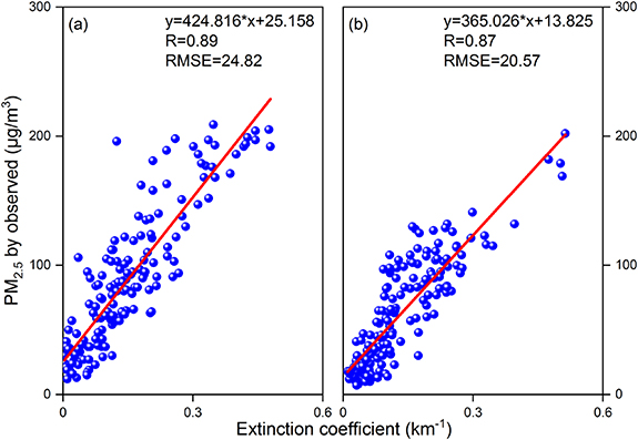
Figure 2. Linear analysis of the aerosol extinction coefficient at 0.1 km and the PM2.5 mass concentration measured in (a) Shijiazhuang and (b) Baoding. The red line is the fitting curve between the extinction coefficient and the PM2.5 concentration.
Download figure:
Standard image High-resolution image2.4. Model and DA system
2.4.1. Modeling of regional PM2.5 production
The WRF-Chem chemical transport model (version 3.8.1) was used to investigate the PM2.5 concentration. Figure S1 shows the model configuration with three nested domains with 100 × 100 (d01, 36 km), 103 × 103 (d02, 12 km), and 151 × 127 (d03, 4 km) grids, and the center was located at 36.228 N, 111.278 E. All of the domains had 101 vertical sigma layers from the ground level to the top pressure of 50 hPa. To better simulate the situation within the boundary layer, the resolution of the boundary layer was set higher, and 34 layers were set in the range of 0–2 km. The model time steps were set to 180 s and the output was released every hour. The initial and boundary meteorological conditions were derived from the 6 h National Centers for Environmental Prediction Final Analysis data with 1° × 1° spatial resolution. The anthropogenic emissions were obtained from MEIC data with 0.25° × 0.25° resolution (Zhou et al 2017). Terrestrial biogenic emissions were estimated using the MEGAN model (Chatani et al 2011). The gas-phase chemistry module CBM-Z and the aerosol module Model for Simulating Aerosol Interactions and Chemistry were used in this simulation.
2.4.2. Data assimilation system
The GSI DA system provides a 3DVAR analysis by minimizing the cost function as shown below (Gao et al 2017):
In this equation, x is the analysis vector, xb denotes the background vector, y is an observation vector, B represents the background error covariance matrix, R represents the observation error covariance matrix, and H is the observation operator used to transform model grid point values to observed quantities, which is achieved via interpolation.
The hourly profile PM2.5 concentrations of the two sets of Lidar data within 1 h windows were assimilated. The observation errors of the Lidar data originated from measurement errors and representative errors. The measurement error was computed using  (Schwartz et al 2012, Jiang et al 2013, Gao et al 2017), where obs indicates the observed values. The representative error was computed using
  (Pagowski et al 2014), where
  is the adjustable scale factor,
  is the model grid resolution (we selected 4 km for the domain), and L is the influencing radius (we used 60 km for the Lidar).
Figure 3 shows a comparison of the non-DA, DA, and observed values, in which the observed values of PM2.5 were provided by the China National Environmental Monitoring Center (http://106.37.208.233:20035). These results clearly indicate that the Lidar data were a significant improvement over the simulation results. The correlation values of the non-DA and DA data were 0.74 and 0.86, respectively, representing an increase of 16.2%. Additionally, the RMSEs of the non-DA and DA data were 24.62 and 15.60 µg m−3, respectively, representing a decrease of 36.6%.
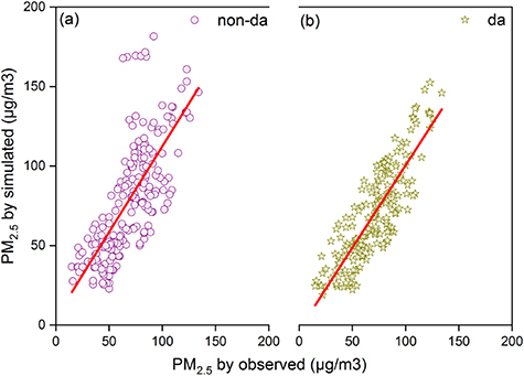
Figure 3. Comparisons of unassimilated and assimilated results of hourly PM2.5 concentrations at multiple sites around in Beijing and its surrounding areas.
Download figure:
Standard image High-resolution image2.4.3. Retrieval method for TF and TFI
Equation (8) was used to calculate the TF of the PM2.5 based on the revised PM2.5 concentration after assimilation and the wind field data from the simulation:

In this equation, PM2.5 (µg m−3) is the concentration of particulate matter at the current height; WS (m/s) and WD are the wind speed and wind direction at the same position, respectively;  represents the angle between the current position and the direction of the transport pathway; and Flux (µg m−2 s−1) represents the TF of the PM2.5 at the current position. Thus, positive values of Flux signify input fluxes, while negative values signify output fluxes. The TFI of the PM2.5 was calculated by integrating the TF of the PM2.5.
3. Results and discussion
3.1. Meteorological conditions
Figure S2 shows the wind field distribution at 4:00 p.m. on 26, 27, and 28 November 2017, which had respective winds from the southeast, southwest, and northwest, and these wind directions at the surface were consistent with those of the upper air. On the North China Plain, the average surface wind speeds for the 3 d were 3.3, 5.0, and 7.6 m s−1, respectively, while the average wind speeds 1 km above the surface were 5.1, 10.7, and 10.9 m s−1, respectively. For Beijing, the average surface wind speeds on the 26th and 27th were < 2 m s−1, causing pollutants to accumulate (Slater et al 2020). Correspondingly, the average upper air wind speeds were > 6 m s−1, which was conducive to the transport of pollutants at upper levels. Meanwhile, the overall wind speeds at both the surface and upper levels in Beijing were relatively high on the 28th, which was conducive to the diffusion of pollutants by the northwest winds.
3.2. Particle extinction coefficient
The Fernald method was used to invert the Lidar data, thereby obtaining the extinction coefficient profile (Lv et al 2016). As shown in figure 4, the particles were mainly concentrated below 1.8 km during the observation period, appearing in decoupled layers. Additionally, the data obtained by the two Lidar systems exhibited good consistency. The maximum extinction coefficient was 1.2 km−1, which occurred at 0.8 km. The stratification of the upper-air and surface pollutants had disappeared by 5:00 p.m.
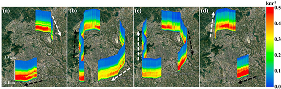
Figure 4. Spatial distribution of aerosol extinction at (a) 2:00 p.m., (b) 3:00 p.m., (c) 4:00 p.m., and (d) 5:00 p.m. on 27 November 2017.
Download figure:
Standard image High-resolution imageIn order to further examine the paths of pollutant transport, figure 5 shows the observation results of the extinction coefficient for the five ground-based Lidars on the North China Plain from 26–29 November 2017. We found that pollutants began to accumulate in Shijiazhuang, Baoding, and other areas in the early morning of the 26th. Meanwhile, under the influence of the southwest wind, pollutants began to travel in the direction of Shijiazhuang, Baoding, and Beijing, with the transport height increasing from 0.6 km in the morning to 1.6 km at night, resulting in high concentrations of pollution in Beijing, Langfang, and other cities. The height of the pollutants began to decrease during the day on the 27th, with the pollutants reaching their peak values on the night of the 27th and in the early morning of the 28th, and the maximum extinction coefficient exceeding 1.5 km−1. During the day on the 28th, under the action of northwest winds, pollutant advection began from north to south. The pollutants in Beijing, Tianjin, Langfang, and Baoding were successively reduced, while the pollutant diffusion conditions in Shijiazhuang were relatively poor due to the low wind speed.
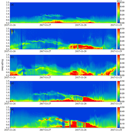
Figure 5. Continuous observation results of ground-based Lidar from 26–29 November 2017: (a) Beijing, (b) Baoding, (c) Shijiazhuang, (d) Langfang, and (e) Tianjin.
Download figure:
Standard image High-resolution image3.3. PM2.5 mass concentration
Figure 6 presents the spatial distribution of the PM2.5 concentration after DA using the two sets of Lidar data. At 2:00 p.m., the PM2.5 appeared in decoupled layers, of which the heavily polluted layer was 200–700 m. At the same time, a layer of low-concentration pollution appeared, ranging from 700–1700 m. These findings are consistent with the Lidar observation results, confirming that the results of the Lidar assimilation system were correct. At 2:00 p.m., the PM2.5 concentration in northwest Beijing was high, with an upper air concentration of 135 µg m−3; the surface concentration, however, was only about 30 µg m−3. When combined with the meteorological results from the WRF-Chem simulation, an updraft near the ground was revealed, which caused the pollutants to spread out into the ambient atmosphere. Hence, the concentration of pollutants near the ground was low. Under the influence of the southwest wind flow, pollutants ahead of the Taihang Mountains were transported to Beijing, causing the PM2.5 concentration in southwest Beijing to reach its maximum at 5:00 p.m. At the same time, the pollutant height decreased, causing the PM2.5 concentration at the surface to reach 126 µg m−3. Meanwhile, in order to further estimate the possible sources and transport pathways of the aerosols, the backward and forward trajectory analyses from the HYSPLIT model are presented in figure S3.
3.4. TF of PM2.5 and TFI of PM2.5
Figure 7 shows the TF results of PM2.5 along the 6th Ring Road in Beijing. A positive TF indicates that PM2.5 was transported to Beijing; otherwise, the pollutants were exported from Beijing. Both the southern portion and the western portion of the 6th Ring Road primarily received PM2.5 during the observation period, with the transmission occurring at 1 km. At the same time, the transmission intensity along the southern part of 6th Ring Road was higher than that along the western part of 6th Ring Road. In the northeast region of Beijing, PM2.5 was mainly transmitted to other cities, and the transmission height was similar to that of PM2.5 transported to Beijing in the southwest region, although the output intensity was significantly lower than the input intensity. The maximum PM2.5 transmission values of 931 and − 701 µg m−2 s−1 in the southern and eastern parts of the 6th Ring Road, respectively, both occurred at 4:00 p.m. Moreover, figure S4 shows the TFI results of PM2.5 along the 6th Ring Road in Beijing. The TFI values of PM2.5 in the eastern, southern, western, and northern parts were −1133, 847, 1060, and −457 µg km−1 s−1, respectively, indicating that pollutants were transported from the southwest to Beijing and diffused from Beijing to the northeast.

Figure 6. PM2.5 concentration (unit: µg m−3) along the 6th Ring Road, Beijing. The x-axis is (a–h) latitude and (i–p) longitude in degrees. The y-axis is the height in meters. The locations represented by east, west, south, and north in the upper left corner correspond to the locations labeled in figure 1.
Download figure:
Standard image High-resolution image
Figure 7. The same as figure 6 but for TF results (unit: µg m−2 s−1) of PM2.5 along the 6th Ring Road, Beijing.
Download figure:
Standard image High-resolution image
4. Conclusion
Accurately quantifying the distribution of particulate matter in the atmosphere is the key requirement for the prediction of air quality and the estimation of atmospheric environmental capacity. In this study, the PM2.5 data from the inversion of seven Lidars (two vehicle-mounted and five ground-based) along with simulated PM2.5 data from the WRF-Chem were coupled to a GSI 3DVAR assimilation system. The PM2.5 field was obtained after the observation data were corrected. When compared with the unassimilated results, the correlation of the DA results based on the Lidar data increased by 16.2%, while the RMSE decreased by 36.6%. Moreover, an analysis of the TF and TFI of the PM2.5 revealed that the PM2.5 along the 6th Ring Road of Beijing was mainly concentrated below 1.8 km, and there were obvious decoupled layers of particles. Particulates in the southwest were mainly input, while those in the northeast were mainly output. Both the input and output heights were around 1 km, although the input intensity was higher than the output intensity.
In addition, the discovery of the aerosol vertical characteristics on the North China Plain has numerous potential applications. Obviously, this dataset can be used to further verify and improve the representation of aerosols in air quality models and satellite remote sensing. In addition, the determination of the aerosol transport characteristics at different heights can provide evidence to explain the cross-border transport mechanism of pollutants. Moreover, the results of the data of this study can also provide technical support and services, which can be utilized by environmental management departments to evaluate the efficiency of pollution control, predict the impacts of air pollution on environmental health, and effectively carry out environmental management and pollution control.
Acknowledgments
This work was supported by the Natural Science Foundation of Anhui Province, China (1908085QD160, 1908085QD170), the National Research Program for Key Issues in Air Pollution Control (DQGG0102), the National Natural Science Foundation of China (41941011), the National Key Project of MOST (2017YFC0213002, 2018YFC0213101, 2016YFC0200401), and the Doctoral Scientific Research Foundation of Anhui University (Y040418190).
Data availability statement
The data that support the findings of this study are available from the authors upon request. The FNL data are available from the following website (https://rda.ucar.edu/datasets/ds083.2/). The data in this study were analyzed using the NCAR Command Language (http://www.ncl.ucar.edu/). The authors are grateful to the China National Environmental Monitoring Center for providing monitoring data for the PM2.5 (http://106.37.208.233:20 035). The authors gratefully acknowledge the NOAA Air Resources Laboratory (ARL) for providing the HYSPLIT transport and dispersion model (https://ready.arl.noaa.gov/HYSPLIT_traj.php) used in this research.