

Abstract
The role of climate and aclimatic factors on species distribution has been debated widely among ecologists and conservationists. It is often difficult to attribute empirically observed changes in species distribution to climatic or aclimatic factors. Giant pandas (A. melanoleuca) provide a rare opportunity to study the impact of climatic and aclimatic factors, particularly the food sources on predicting the distribution changes in the recent decade, as well-documented information on both giant panda and bamboos exist. Here, we ask how the climate metrics compare to the bamboo suitability metric in predicting the giant panda occurrences outside the central areas in the Qinling Mountains during the past decade. We also seek to understand the relative importance of different landscape-level variables in predicting giant panda emigration outside areas of high giant panda densities. We utilize data from the 3rd and 4th National Giant Panda Surveys (NGPSs) for our analysis. We evaluate the performance of the species distribution models trained by climate, bamboo suitability, and the combination of the two. We then at 4 spatial scales identify the optimal models for predicting giant panda emigration between the 3rd and the 4th NGPSs using a list of landscape-level environmental variables. Our results show that the models utilizing the bamboo suitability alone consistently outperform the bioclimatic and the combined models; the distance to high giant panda density core area and bamboo suitability show high importance in predicting expansion probability across all four scales. Our results also suggest that the extrapolated bamboo distribution using bamboo occurrence data can provide a practical and more reliable alternative to predict potential expansion and emigration of giant panda along the range edge. It suggests that restoring bamboo forests within the vicinity of high giant panda density areas is likely a more reliable strategy for supporting shifting giant panda populations.
Export citation and abstract BibTeX RIS
1. Introduction
Giant Panda (A. melanoleuca), one of the most charismatic wildlife species in the world, commands tremendous public interest and conservation resources (figure 1). Although its IUCN Red List status was recently downlisted from endangered to vulnerable, the giant panda population still faces many challenges including climate change, habitat loss, and fragmentation driven by anthropogenic disturbances (Swaisgood et al 2018).
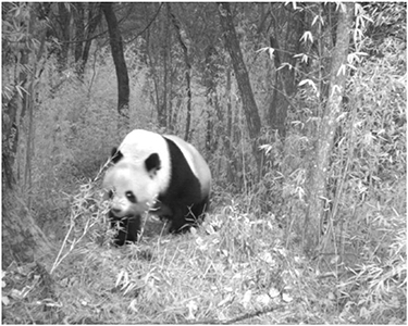
Figure 1. Camera trap photo of a giant panda in Guanyinshan reserve in Qinling mountains.
Download figure:
Standard image High-resolution imageMultiple studies have predicted drastic changes in giant panda's future distribution (Tuanmu et al 2012, Songer et al 2012, Wang et al 2018). However, predictions vary greatly due to the choice of analytical tools, the uncertainty of climate change scenarios, complex interactions among giant pandas, bamboo, and various environmental constraints (Huang et al 2018b). It is generally agreed upon that climate serves as a key constraint of species distribution over the long term by shaping their potential niche. In contrast, the availability and spatial distribution of aclimatic factors, particularly biotic forces such as food resources, predation, competition can significantly influence a species' realized niche (Hijmans and Graham 2006, Pearson and Dawson 2003, Heikkinen et al 2006, Araújo and Luoto 2007). However, it is often not clear empirically observed changes in species distribution are driven by climatic or aclimatic factors. Giant panda, in particular, has a direct and close association with bamboo distribution because of its strict dependency on bamboo as its sole food source (Wang et al 2018, Huang et al 2018a, Tian et al 2019). Bamboo comprises over 99% of the diet of giant pandas. Though giant pandas forage primarily on vegetation, their gut anatomy resembles that of a carnivore, with a simple stomach and short gastrointestinal tract, which results in their requirement of consuming large quantify of bamboo to maintain their nutritional needs (Huang et al 2018a). Notably, in Qinling, giant panda also migrates to higher elevation areas in summer and stays in lower elevation areas over winter, a pattern correlates closely with temperature variation (Loucks et al 2003). Comparing influences between climate change and bamboo on giant panda distribution can help elucidate the complex interplay between climatic and non-climatic factors. It is not clear, however, how climate change compares to bamboo distribution in predicting the observed shift of giant panda distribution in the recent decade.
Effective management and restoration of giant panda habitat hinge on our ability to thoroughly examine and attribute the recent changes in giant panda distribution. Changes in species distribution can sometimes be an adaptive mechanism to track suitable climatic space in response to rapid changes in climatic conditions (Tingley et al 2009). Alternatively, it could also be density-dependent dispersal that is driven by suitable habitat conditions and less competition in surrounding areas (Matthysen 2005). As giant panda population grows (State Forestry Administration of China 2006, Swaisgood et al 2018), additional corridors and protected areas need to be established, and habitat needs to be restored to support the expansion (Zhang et al 2019). Determining the drivers of changing giant panda distribution is of paramount importance to facilitate those conservation planning and practices.
Aside from variable climate conditions, many aclimatic factors play critical roles in determining whether animals can emigrate outside of the established suitable habitat. Factors such as dispersal cost (affecting the difficulties of emigrating from one point to the other, e.g. distance, connectivity, physical barriers, the variability of elevation) (Rousset and Gandon 2002, Baguette and Van Dyck 2007, Bonte et al 2012), habitat condition (Wang et al 2008, Huck et al 2010), and presence of anthropogenic disturbances (Theobald et al 1997, Apps and McLellan 2006), and protection status of landscapes (closely associated with both the habitat condition and anthropogenic disturbance) can have significant impacts on the ability of animals to emigrate. They thus can be managed proactively to facilitate adaptive conservation management. Such analysis can be conducted independently regardless of variable climate predictions, and thus can provide practical and actionable management insight for wildlife managers and policymakers. There is an urgent need to examine what landscape-level environmental factors, aside from climatic conditions, drive the expansion of giant panda distribution.
The National Giant Panda Surveys (NGPS) conducted by the Chinese government provide an unprecedented opportunity to examine the recent changes in giant panda distribution over a large geographical scale. The 3rd and the 4th NGPSs are the most recent surveys, which were conducted during 2001–2003 and 2011–2014, respectively (Swaisgood et al 2018, Wei et al 2018). Tremendous amounts of resources have been spent on conducting surveys covering extensive areas (Zhang et al 2011, Wei et al 2018). The survey results not only documented detailed giant panda signs over large areas but also included information on bamboo distribution which are valuable assets for examining the spatial relationships between bamboo availability and giant panda distribution.
The Qinling Mountains in Shaanxi province have the highest giant panda density among all 6 mountain ranges (State Forestry Administration of China 2006). Giant panda distribution has undergone changes between the 3rd and the 4th surveys in Qinling (see population change over the past surveys in the supplementary data files stacks.iop.org/ERL/15/084036/mmedia); specifically, giant pandas have been spotted in recent years in many areas that historically had no or few pandas, primarily in the peripheral of known range. The minimum giant panda population estimate reported by the latest two surveys has gone from 273 to 345 (20% increase over 10 years) (supplementary data files). The emigration of the giant pandas outside of traditionally high-density areas has been spatially heterogeneous. Although much of the 4th survey data related to giant panda occurrence within the central areas of the Qinling Mountains remains unavailable due to data sharing policies and restriction, the peripheral data has been made available. The available data provides a rich source for validating the accuracy of various species distribution models, parameterized by combinations of climatic and bamboo suitability metrics. Furthermore, the giant panda occurrence data outside of the central area also provide a unique opportunity to evaluate the importance of various aclimatic environmental variables for predicting the probability of expansion and emigration.
In this study, we seek to answer two main research questions: (1) How do the climate change metrics compare to bamboo availability metrics in terms of their efficacies in predicting the giant panda expansion outside the central areas in the Qinling Mountains during the past decade? (2) What is the relative importance of different landscape-level variables in predicting emigration probability outside areas of high giant panda densities?
We first built species distribution models utilizing the full set of giant panda occurrence data of the 3rd NGPS across the Qinling Mountains. The combinations of climatic and bamboo metrics were used to train the contrasting models. The models' performance is then evaluated and compared using the available giant panda occurrence observed from the 4th NGPS outside of the central areas. To answer the second question, we first identified the giant panda emigration points comparing both the 3rd and 4th NGPS data. We then identify the optimal model for predicting emigration ability within grid cells at various scales using a list of landscape-level environmental variables. Finally, we examine the composition of the optimal model and the importance of different variables across scales.
2. Data & method
2.1. The performance of climatic- & bamboo- models
2.1.1. Study area and species occurrence data
The study area is in the Qinling Mountains in Shaanxi Province, located in northwest China. Qinling is one of the six mountain ranges where wild giant pandas are currently present (see map of study area in supplementary data files). Based on the result of the 4th NGPS, Qinling has the highest giant panda density among all six mountain ranges, with 345 individuals identified within its range.
Based on availability, we used giant panda occurrence data covering the full Qinling range from the 3rd survey and the one covering part of the Qinling from the 4th survey for analyses. The available giant panda data from the 4th NGPS was outside the central Qinling area. The central Qinling is conventionally referred to as the area in the south slope of the Qinling Mountains, partially including a few well-established giant panda nature reserves such as Changqing, Foping, Huangbaiyuan, and Laoxiancheng, supporting the highest density of giant pandas. The dataset provides an opportunity to examine the latest giant panda distribution at the periphery of the Qinling Mountains and to validate various distribution model predictions.
We also obtained bamboo occurrence data across the entire Qinling surveyed from the 3rd and the 4th NGPSs.
2.1.2. Species distribution model setup
We constructed three Maxent species distribution models (Phillips et al 2006) for comparison purposes: a traditional bioclimatic model, composed of 19 bioclimatic variables and elevation (Songer et al 2012), a bamboo-only model, with just a bamboo suitability layer, and a combined model, including all variables from the other two models. To reduce the collinearity among variables, between pairs of variables with an absolute correlation coefficient larger than 0.5, we only kept the variable with the higher jackknife variable importance measure. The models were first trained using predictive variables extracted at the giant panda occurrence (n = 1564) collected during the 3rd NGPS. Ten thousand background points were created for each Maxent model to capture the environmental gradient (Phillips et al 2006, Kumar and Stohlgren 2009, Dudik et al 2010). The models were then projected into the following decade using the updated climate and bamboo data. Lastly, the projected giant panda distributions were tested using a subset of giant panda signs (n = 576) collected during the 4th NGPS which were outside the central area of the Qinling Mountains.
2.1.3. Climatic data
To generate climatic variables, we used CHELSA climate dataset with 30 arc sec (∼1000 m) resolution to quantify climate conditions in two decades (Karger et al 2017). Nineteen bioclimatic variables around the time of the 3rd NGPS were calculated as the baseline climate conditions. The 10 year (1994–2003) and 5 year (1999–2003) means of the bioclimatic variables were computed to average out the short term variability of climatic fluctuation. We used the averaged bioclimatic variables as predictors in the bioclimatic models and the combined models. We also fed the bioclimatic data around the time of the 3rd and 4th NGPS to the bamboo distribution models to extrapolate bamboo suitability.
2.1.4. Bamboo suitability index
We used the Maxent model to generate wall-to-wall maps of the bamboo suitability index (ranging between 0 and 1) to be used as predictive variables. We combined surveyed bamboo occurrence data from the 3rd (n = 1804) and 4th NGPS (n = 5998) and the CHELSA bioclimatic data. To be consistent with other models and climatic variables, the bioclimatic variables were averaged with the same 5-year and 10-year windows around each survey period. For each averaging window and for each survey period, we trained the model with the bamboo occurrence and corresponding bioclimatic variables and then extrapolated a suitability index across the entire area.
2.1.5. Model comparison
The output was a total of 6 contrasting models (2 averaging windows × 3 models (the bioclimatic, bamboo-only, and combined model)). We built the model with dismo (Hijmans et al 2015) package in R (R Development Core Team 2011). The model results, the gridded maps of giant panda occurrence probability (ranging from 0 to 1), were tested against the 4th NGPS giant panda occurrence using area-under-curve (AUC) metrics. The model results were grouped by the temporal window size and compared within groups.
2.2. Importance of the aclimatic variables in expansion models
2.2.1. Model setup
To compare the importance of aclimatic variables in contributing to giant panda expansion and emigration, we first delineated the high giant panda density core area and then identified expansion locations. To understand the sensitivity of scales to the results, we created 4 grid systems with different resolutions. The presence and absence of the expansion points among grid cells outside the core areas were modeled using a logistic regression model with a list of environmental variables (see Environmental Variables section below). The variables are designed to capture different aspects of dispersal cost, protection status, habitat conditions, and anthropogenic disturbances.
2.2.2. Expansion points
To delineate the expansion points, we first delineated the high-density core area boundaries. The boundary of the core area was drawn by fitting a kernel density estimation over the giant panda occurrence from the 3rd NGPS, which contained 99% of 3rd NGPS occurrence points using a plug-in bandwidth selector to determine kernel smoothing (figure 2). The plug-in bandwidth selector was chosen because it has been shown to be as accurate as or more accurate in identifying home-range than other bandwidth selectors for locating distributions of detection data (Gitzen et al 2006, Downs and Horner 2008). We then identified the expansion points as the giant panda occurrence from the latest 4th NGPS outside of the high-density core areas (figure 2). The process resulted in 73 expansion points outside of the core areas.

Figure 2. The expansion points delineation. The top panel (a) shows the giant panda occurrence points documented by the 3rd National Giant Panda Survey (NGPS). The high-density core area boundary (red line) delineated by fitting a kernel density estimation over the 3rd NGPS detections. The area contains 99% of the detected 3rd NGPS occurrence data (black points) using a plug-in bandwidth selector. The lower panel (b) shows the high-density core area boundary and the identified expansion points. The points are defined as the giant panda occurrence from the latest 4th NGPS outside of the high-density core areas. The hatched areas in both panels show the distribution of existing protected areas.
Download figure:
Standard image High-resolution image2.2.3. Grid systems
The area outside the delineated core area in Qinling Mountains was divided into grids. The presence and absence of the expansion points were modeled at the grid cells level within which a list of aclimatic environmental indices was aggregated and used as predictive variables. The spatial scale of the grid influences the way environmental variables are aggregated and can often lead to significant variability in distribution modeling (Saupe et al 2012). To examine the impact of scale on the models, we created 4 grid systems with cell size of 12 km, 6 km, 3 km, and 1 km. The 4 different resolutions were selected because they covered a spectrum of distances between giant panda's lifetime dispersal distance (∼12 km) (Zhan et al 2007, Hu et al 2010), seasonal migration distance (∼6 km) (Liu et al 2002, Zhang et al 2014), and daily foraging distance (∼1 km) (Zhang et al 2014). As a result, the process created 18, 28, 36, 56 presence grids and 198, 828, 3409, and 30 918 absence grids accordingly.
2.2.4. Environmental variables
Aside from dispersal cost and bamboo availability which are directly related to giant panda's dispersal, indices related to anthropogenic disturbances (Qi et al 2007, Wang et al 2014), habitat fragmentation (Yang et al 2017), and terrain condition (Liu et al 2005, Wang et al 2018) were also selected as predictive variables in the expansion model (table 1), because they have showed efficacies in affecting giant panda habitat suitability. At each scale and for each grid cell, we quantified 10 aclimatic environmental variables to serve as the predictive variables. For each pixel cell, we characterized the dispersal cost by calculating the nearest Euclidean distance to the 3rd NGPS giant panda occurrence points, the nearest distance to the high-density core area, and the Terrain Roughness Index (TRI) which was calculated as the mean of the absolute differences between the elevation value of a cell and its 8 surrounding cells. We calculated the TRI from 90 m- resolution digital elevation data based on 2000 Shuttle Radar Topography Mission (Reuter et al 2007). The average variable values were aggregated within every grid cell at each spatial scale.
Table 1. The landscape-level aclimatic variables used for the expansion models.
| Name | Description | Unit |
|---|---|---|
| 3rd Survey Distance | Euclidean distance to nearest giant panda sign of the 3rd Survey | m |
| Core Distance | Euclidean distance to core area of the 3rd Survey | m |
| Reserve Area | Area of protected land | m2 |
| Interior Forest Area | Total area of interior forest (pixels not directly adjacent to forest edge) within a raster cell in the year 2012 | m2 |
| Average Forest Patch Size | Average area of forest patches in the year 2012 per raster cell | m2 |
| Average Amount of Forest Edge | Average number of forest edge pixels per forest patch within a raster cell in the year 2012 | Count of 30 m2 cells |
| Predicted Bamboo Suitability | Predicted suitability for bamboo, as predicted by a Maxent model fit to 4th Survey bamboo locations, and environmental variables from the 10 years around the 4th Survey. | Probability of presence |
| Average Terrain Roughness | Average Terrain Roughness Index value per grid cell | Unit-less |
| Distance to High Night-time Light | Euclidean distance to the nearest area with night-time light greater than or equal to the 3rd quartile value of night time light detected in the Qinling region. | m |
| Distance to Roads | Euclidean distance to the nearest roadway | m |
We then calculated the area of reserve per grid cell, average bamboo suitability, total area of interior forest area (forested pixels not directly adjacent to forest edge), average forest patch size, and average amount of forest edge per patch within each grid cell (table 1). We used the bamboo suitability layer around the 4th NGPS with 10-year averaging window. For the forest-related metrics, we first used forest cover map at 30 m resolution of the year 2012 (Hansen et al 2013) to define forest and non-forest pixels. We then used SDMTools package (Van Der Wal et al 2014) in R to compute the amount of interior forest area, forest patch size, and forest edge per patch within each grid.
We used two metrics to characterize the intensity of anthropogenic disturbance (table 1). The distance from a specific location to high night-time light areas is considered a good indicator of human population density and intensity of disturbance (Hull et al 2014). We used the third quantile value of all night-time light cells in the Qinling Mountains as a threshold to define high night-time light areas. The night-time light data is based on the DMSP-OLS Night-time Lights Time Series Version 4 (∼1 km resolution) for the year 2012 (Elvidge et al 1999). We calculated the mean distance to the nearest major roadway for each pixel cell using road network data from the Open Street Map network of China (OpenStreetMap 2017). Finally, we aggregated the mean values of both anthropic disturbance variables within the grids of different scales.
2.2.5. Variable selection & variable importance
To reduce collinearity among model variables, at each scale, we computed the pair-wise Kendall rank correlation coefficient between 10 variables. We used the individual variables in logistic regression models to predict the presence and absence of expansion occurrence. We documented the Akaike information criterion (AIC) values for the single-variable models as a way to quantify individual variable predictability. Between pairs of variables with an absolute correlation coefficient larger than 0.5, we kept the variable with the lower AIC value. We used the dredge function in the MuMIn R package (Barton and Barton 2015) to fit the models with all possible combinations of predictive variables. The best models were selected based on AICc value (AIC corrected for small sample size).
For each model, ΔAICc measures the increase of AICc values (decrease of performance) compared with the best models. We documented in supplementary data files the lower-ranking models as alternative models when the ΔAICc <0.5 (Kaiser-Bunbury et al 2017).
For each predictive variable, we aggregated AIC-weight over all possible models in which the variable was included. The resulted unit-less metric is a variable importance measurement; the metric ranges between 0 and 1, where the index showed lowest (weakest explanatory ability) and highest importance (strongest explanatory ability), respectively (Borer et al 2014, Barton and Barton 2015).
3. Results
3.1. Species distribution model predictions evaluation
The models utilizing the bamboo suitability layer as the only predictive variable consistently outperformed the bioclimatic models. The bamboo models also consistently had slightly better predictability than the combined models encompassing both bamboo and bioclimatic variables. With the 5-year climate average, the bamboo-only model produced the highest AUC value of 0.938, followed closely by the combined model with an AUC of 0.932, and the bioclimate model with AUC of 0.899 (table 2). With the 10-year climate average, the trend persisted: the bamboo-only model performs the best with an AUC value of 0.927, followed by the combined model with a slightly lower AUC of 0.923, and the bioclimatic model with an AUC of 0.85 (table 2).
Table 2. Species distribution models performance comparison.
| Model | AUC | Predictive Variables Used |
|---|---|---|
| 5 year average, bamboo only | 0.938 | Predicted bamboo suitability |
| 5 year average, bioclimatic variables | 0.899 | Elevation, mean diurnal range, temperature annual range, precipitation seasonality |
| 5 year average, combined model | 0.932 | Predicted bamboo suitability, mean diurnal range, temperature annual range, mean temperature of wettest quarter, precipitation seasonality, precipitation of warmest quarter |
| 10 year average, bamboo only | 0.927 | Predicted bamboo suitability |
| 10 year average, bioclimatic variables | 0.85 | Elevation, mean diurnal range, temperature annual range, precipitation seasonality |
| 10 year average, combined model | 0.923 | Predicted suitability of bamboo, mean diurnal range, temperature seasonality, precipitation seasonality, precipitation of coldest quarter. |
3.2. Expansion probability models variable selection and variable importance
The 4 expansion models at various scales were initiated with slightly different sets of predictive variables controlling for pair-wise correlation among variables. At all scales, distance to the core areas is highly correlated (>0.7) with distance to the nearest sign from the previous survey; the amount of interior forest is also highly correlated with average forest edge and average patch size. Thus, distance to the nearest sign from the 3rd NGPS, average forest edge, and the average patch size were not included in all models. One exception was that the average forest edge,being included in the model at 1 km scale (table 3).
Table 3. The expansion model setup and the optimal model composition at different scales.
| Scale | Predictive Variables | Significant Variable | Estimate | Standard Error (±) | p-Value |
|---|---|---|---|---|---|
| 12 km | Core Distance, Reserve Area, Area of Interior Forest, Bamboo Suitability, Terrain Roughness, Distance to High Night Time Light, Distance to Roads | ||||
| Core Distance | −4.00 | 1.53 | 0.01a | ||
| Interior Forest Area | 5.26 | 2.15 | 0.01a | ||
| Bamboo Suitability | 1.11 | 0.55 | 0.04a | ||
| Distance to Road | −0.47 | 0.33 | 0.15 | ||
| 6 km | Core Distance, Reserve Area, Area of Interior Forest, Bamboo Suitability, Terrain Roughness, Distance to High Night Time Light, Distance to Roads | ||||
| Core Distance | −2.82 | 0.76 | <0.01a | ||
| Bamboo Suitability | 2.03 | 0.47 | <0.01a | ||
| Distance to High Night Time Light | 0.48 | 0.25 | 0.05a | ||
| 3 km | Core Distance, Reserve Area, Area of Interior Forest, Bamboo Suitability, Terrain Roughness, Distance to High Night Time Light, Distance to Roads | ||||
| Core Distance | −2.46 | 0.61 | <0.01a | ||
| Bamboo Suitability | 2.21 | 0.43 | <0.01a | ||
| Distance to High Night Time Light | 0.41 | 0.21 | 0.06 | ||
| Distance to Road | −0.30 | 0.17 | 0.07 | ||
| 1 km | Core Distance, Reserve Area, Area of Interior Forest, Bamboo Suitability, Terrain Roughness, Distance to High Night Time Light, Distance to Roads, Average Amount of Forest Edge | ||||
| Core Distance | −2.81 | 0.54 | <0.01a | ||
| Bamboo Suitability | 2.48 | 0.38 | <0.01a | ||
| Distance to High Night Time Light | 0.49 | 0.17 | 0.01a | ||
| Terrain Roughness | −0.48 | 0.21 | 0.02a | ||
| Distance to Road | −0.20 | 0.13 | 0.13 |
aRepresent a significant coefficient with significance level of 0.05.
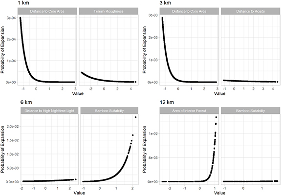
The optimal models resulting from the dredge process had a few common variables shared across scales. The distance to core giant panda area was consistently included in optimal models across 4 scales, showing a negative correlation with expansion probability; the extrapolated bamboo suitability was also selected in all final models, exhibiting a positive correlation with expansion probability (table 3). The two variables had significant coefficients in all models in which they were included. Distance to high night-time light area was significant in 3 final models (at 6 km, 3 km, 1 km scales) and had a positive correlation with the expansion probability. Distance to roads was included in the best models at 12 km, 3 km, and 1 km scales; it had a negative correlation with expansion probability, but the coefficients were not significantly different from zero. The terrain roughness was included in the optimal model at 1 km scale, exhibiting a significantly negative coefficient; the interior forest was included in the optimal model at 12 km scale, with a significant and positive coefficient.
The variable importance measures, in general, were consistent with the variable selection process. The distance to high giant panda density core area and bamboo suitability consistently showed high importance (≥ 0.65) in the expansion models across all scales (figure 3). Distance to high night-time light also showed high importance for the models at 1 km and 3 km scales. The amount of interior forest and the distance to the nearest giant panda occurrence from the previous national survey also had high importance, but only for the model at 12 km scale. Terrain roughness and distance to the nearest road exhibited high importance at models at 1 km and 3 km scales, respectively.
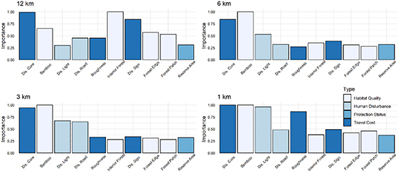
Figure 3. The measure of importance of environmental variables in expansion models at 4 different scales.
Download figure:
Standard image High-resolution image4. Discussion
The under representation of biotic factors in species distribution models has been widely discussed (Heikkinen et al 2006, Araújo and Luoto 2007, Wang et al 2018). For most species, it is relatively difficult to answer, firstly, what constitutes key biotic factors and, secondly, how biotic factors can be incorporated in the modeling process. It is also rare to have data for both the species of interest and the species that exerts strong biotic interactions. Thus, few studies have empirically evaluated the impact of biotic interactions on recent changes in species distributions. Our study on giant pandas provides a unique opportunity to tackle the issue because of its strict bamboo diet as well as the extensive data generated from the National Giant Panda Surveys on both giant panda and bamboo.
Our study compared the effectiveness of models utilizing bamboo suitability and climate conditions, and the combined models by validating the models with the occurrence data from the latest 4th NGPS. Although the validation data used to test the model accuracy, covering areas outside the central Qinling areas, was a subset of the entire dataset, it is advantageous to test model performance using the data from outermost limit of giant panda range. Those are the areas where changes in giant panda distribution are most likely to occur (Songer et al 2012). Environmental conditions at the range edges often pose as physical limitations to species survival and reproduction, preventing the species from spreading further. For most species, the outermost limit of the range is where they are most sensitive to changing environmental gradients, and where the most prominent distribution shifts happen under climate change scenarios (Parmesan et al 1999, Gaston 2003, Huang et al 2016). Our study provides an example demonstrating that a partial dataset like this can still be tremendously useful in validating species distribution change models and providing insights on the driving forces of distribution changes.
Our results showed that the single variable of bamboo suitability is a superior predictor compared to multidimensional characterization of climate conditions in predicting recent giant panda occurrences outside the central Qinling area. The bamboo only model also performed equally, if not better than the model combining both bamboo and climate data, suggesting that bamboo suitability layer is able to explain most of the model variance. The improvement from adding climate information is marginal. The variable importance measure (supplementary data files) also confirmed that bamboo suitability have stronger explanatory ability than other environmental variables: the variable was ranked as the most important in both models that combine climate and bamboo variables; it also has significantly higher permutation importance value than any other environmental variable (supplementary data files). The results suggest that given the temporal scale of the study, the habitat-specific aclimatic factors might be more reliable in predicting changes in species distribution than climate conditions. The improved performance of models with bamboo suitability layers could be attributed to the process in which they have been parameterized by a large number of bamboo occurrence data. Since bamboos are common across the landscape and relatively easy to survey, the process can leverage large quantities of bamboo occurrence data and extrapolate the distribution with less uncertainty (Huang et al 2018b). Our results suggest that the modeled bamboo distribution, which is a more effective proxy to giant panda distribution, can provide a practical and more reliable alternative to predict potential expansion and emigration of giant panda into peripheral areas or emerging habitat.
Admittedly, the distributions of all species, including bamboo, are affected by climate over the long term. However, the debate over the impact of biotic factor (one of the main aclimatic variables that determine species distribution), or the lack thereof in species distribution model focuses on the fact that the biotic factors (e.g. bamboo distribution) often are not in alignment with the shift of climatic niche (Pearson and Dawson 2003, Brooker et al 2007, Araújo and Luoto 2007). The species exerting biotic impact might operate on a set of unique relationship with climate and a range of aclimatic factors. Here, we addressed the issue by building separate species distribution models parameterized on a large number of bamboo occurrences documented by each survey coincidental with giant panda data. It enabled us to fulfill our objective to compare the influence of climate and bamboo. It also allowed us to examine which one of the two is more reliable and practical indicator in predicting giant panda expansion, even though bamboo distribution might be linked with climate to certain degree and through different mechanisms.
Our results have practical implications for giant panda habitat conservation and restoration. The results suggest that restoring bamboo forests within the vicinity of high giant panda density areas is likely a more reliable strategy for supporting shifting giant panda populations compared to prioritizing areas identified through projected suitable future climate conditions.
Currently, most of the bamboo maps are produced to some extent with the help of ground observations, remote sensing data, sophisticated machine learning models, and aided by ancillary environmental data layers (Wang et al 2009, Tuanmu et al 2010, Ghosh and Joshi 2014). It remains challenging to separate bamboo, particularly understory bamboo forest from non-bamboo-forest, based solely on traditional passive remote sensing data; because the spectral signatures of bamboo forests are extremely similar to that of the general forest. The existing bamboo maps also have limited temporal coverage. That is in part what led to our decision to utilize species distribution model approach instead of relying on remotely sensed bamboo maps. However, in the near future, the space-born active remote sensing sensors such as the one used in the NASA GEDI mission (Dubayah et al 2020) have the potential to detect three-dimensional vegetational structure over broad areas and thus could produce more accurate bamboo maps across giant panda habitat for more informed conservation planning.
Previously, many studies have examined the spatial pattern of wildlife expansion. However, the quantitative method to define expansion is scarce. Some of the studies focused on reintroduced or invasive species, where the range expansion can be easily defined as the occurrence outside of known release locations (Reynolds 1998, Veech et al 2011, Fasola et al 2011, Whittington-Jones et al 2011, Jung 2017). Similarly, some studies characterized range expansion as species occurrence outside of historic range maps; they had either limited information on how the maps were made (Crozier 2004, Sun et al 2017), or compiled the range maps by fitting historic sighting records, transect or radio tracking records with simple polygon (Messier et al 1988, Livezey 2009). Alternatively, some studies also produced relatively coarse range maps by dividing up study areas into administrative areas (e.g. counties). In such a context, expansion was defined as the consistent sighting of species in previously unoccupied administrative areas (Waithman et al 1999). There is likely no single way of delineating species range and defining expansion, as population around the fringes of the species range fluctuate significantly over time due to local colonization and extinction (Gaston 2003). Nevertheless, our study aims to provide a quantitative way to characterize species range expansion using large scale sign survey data. The choice of using 99% kernel density threshold to delineate high density core area creates a relatively conservative estimate of expansion location (compared with alternative 95% or 90% thresholds), since the resulting core areas leave fewer points outside as expansion points. But we believe that the method allowed us to identify the occurrence located beyond the outermost limit of giant panda range in Qinling and is most suited for our study objectives. Future studies could focus on examining the sensibility of alternative kernel density thresholds on variable importance in expansion models that can potentially shed light on the variability of habitat selection preferences as animals move from established range to novel environment (Duckworth and Badyaev 2007).
An exploratory analysis showed that the general forest cover in Qinling area had limited variability across grid cells and thus did not contribute to differentiating the presence and absence of expansion occurrences. As a result, we selected the amount of interior forest as opposed to total forest cover in our study as one of our predictive variables. The fragmentation metrics such as the amount of interior forest, average amount of forest patches, and forest edges are indicative of the degree of disturbance, habitat connectivity, and overall habitat quality. They are often closely correlated with each other. The results here showed that the amount of interior forest is an important predictor of expansion at 12 km scale, and it is also consistently ranked more influential than the other two fragmentation metrics in predicting expansion probability across scales (supplementary data files). It can be used in the areas with uniformly high forest cover to better differentiate habitat quality. Additionally, one of the advantages of the core forest metrics is that it has a strong positive association with post-disturbance recovery progress as the amount of interior forest would consistently increase as habitat quality improves and recovers. It provides a more straight-forward and more readily interpretable index of habitat quality than measures of patch number, patch size and edge number, many of which could counterintuitively show elevated degree of fragmentation at early stage of habitat recovery often when small and new habitat are emerging (Yang et al 2017).
Research has shown that giant pandas are less likely to be present in areas with anthropogenic disturbances. Our results are consistent with previous studies in showing that their expansion probability decreases when the distance to high intensity of human disturbance decreases (figure 4). However, when it comes to roads, our results show a slightly negative relationship between distance to road and expansion (figure 4). The negative relationship, albeit not significant by a small margin (p-value = 0.07), is rather surprising, since it contradicts with existing understanding of the relationship between giant panda habitat and transportation infrastructure (Wang et al 2014). The result could suggest a small bias in sampling intensity and survey effort towards road accessible areas. With little information available on the survey transects and survey effort of the National Giant Panda surveys, it is beyond the scope of this study to confirm or preclude the possibility of bias. It is, however, a critically important issue to be addressed in future. Improved accessibility to the transect designs and survey effort of the NGPSs is needed to facilitate future studies on potential sampling biases.
Figure 4. The response curves for the selected key variables included in the optimal models at 4 different scales.
Download figure:
Standard image High-resolution image
We found a surprisingly low association between the area of reserve in each grid cell and the probability of expansion. The results suggest that giant pandas do not select against unprotected areas when they emigrate and expand their distributions. However, the areas in the peripheral of Qinling tend to have less protected areas compared with the central Qinling. As giant panda population continues to increase, they will expand into areas with suitable habitat with or without protection status. We urgently need to establish more reserves and extend protection in the areas outside and between existing reserves. It is our recommendation to extend corridors and establishing new protected land, particularly around new reserves established in the early 2000 s. The reserves with relatively short protection history are playing a critical role in connecting emerging habitat and newly established habitat in the eastern and western Qinling to the central areas. For instance, particularly prime locations for establishing new habitat and corridors are around Niuweihe and Huangguanshan reserves, where there are large gaps of protected land around. More importantly, establishing and restoring bamboo forest near existing high-density areas would have high efficacies in facilitating dispersal and providing additional habitat for continued population growth and recovery. Additionally, a standard of assessing the carrying capacity of existing and prospective protected lands will be immensely useful. Such measures, when factoring in resource availability, habitat quality, and existing density of giant panda, will effectively help assess the priority among existing and prospective reserves.
Acknowledgments
We thank Fang Wang for his support in data collection and providing valuable comments for the manuscript. We also appreciate the help from Turner Sydney Langford on data visualization and organization.
Data availability statements
The data that support the findings of this study are available from the corresponding author upon reasonable request.