

Abstract
Conservation tillage is a primary tenet of conservation agriculture aimed at restoring and maintaining soil health for long-term crop productivity. Because soil degradation typically operates on century timescales, farmer adoption is influenced by near-term yield impacts and profitability. Although numerous localized field trials have examined the yield impacts of conservation tillage, their results are mixed and often unrepresentative of real-world conditions. Here, we applied a machine-learning causal inference approach to satellite-derived datasets of tillage practices and crop yields spanning the US Corn Belt from 2005 to 2017 to assess on-the-ground yield impacts at field-level resolution across thousands of fields. We found an average 3.3% and 0.74% yield increase for maize and soybeans, respectively, for fields with long-term conservation tillage. This effect was diminished in fields that only recently converted to conservation tillage. We also found significant variability in these effects, and we identified soil and weather characteristics that mediate the direction and magnitude of yield responses. This work supports soil conservation practices by demonstrating they can be used with minimal and typically positive yield impacts.
Export citation and abstract BibTeX RIS

Original content from this work may be used under the terms of the Creative Commons Attribution 3.0 licence. Any further distribution of this work must maintain attribution to the author(s) and the title of the work, journal citation and DOI.
1. Introduction
Tillage has been a component of global agricultural systems for millennia. Turning over the soil helps control weeds, break up compaction, and mix nutrients [1]. This repeated disturbance, however, produces unnaturally high erosion rates in agricultural fields [2], harms soil biota [3], and damages soil structure [4]. Combined with other soil pressures, this has resulted in widespread degradation [5] and cropland abandonment at rates exceeding 10 million hectares per year over the past century [6–8]. These losses pose a serious challenge to meeting current and future global food demand.
To combat these negative effects, conservation tillage is promoted to restore and maintain soil health for long-term crop productivity. It is characterized by the retention of at least 30% of crop residues on the soil surface and often achieved through low-impact tillage techniques such as no-till or strip till [9]. These residues and reduced soil disturbance help prevent erosion [2], improve water retention and drainage [10, 11], and foster the quantity and quality of organic matter [4, 12, 13]. After emerging in response to the 1930s Dust Bowl in the United States (US), large-scale adoption began in the 1980s and 1990s following the development of modern herbicides and specialized technology [1, 14, 15]. Today, conservation tillage is practiced on over 150 million ha worldwide, with adoption concentrated in South America, Oceania, and North America [14–16].
Because soil degradation typically operates on century timescales, near-term yield impacts and profitability are key factors for farmer adoption [17, 18]. Numerous studies have examined the yield effects of conservation tillage, and their results are mixed. A recent global meta-analysis concluded that no-till reduced yields by 5.1% in aggregate, although substantial variability existed among crops and biomes [16]. While maize yields remained lower regardless of duration, all other crop categories did achieve similar (but not higher) yields to conventional tillage after 5+ years, suggesting an initial yield penalty due to an adjustment period [16]. In contrast, other studies have found no or even positive yield impacts for maize [19–23] along with variable effects by soils, weather, and/or rotation practices [16, 19, 22–24]. Soybean yields are typically found to be indistinguishable among tillage practices [16, 19–21, 25], with some exceptions [26–28].
Ultimately, a paucity of real-world conditions across biophysical gradients in the literature limits insights meaningful for practitioners. Many studies involved small-scale research plots on level ground with good soils, prohibiting the use of field-scale equipment, inclusion of sloped fields, and a range of soil quality, all cases that may favor conservation tillage [16, 29]. Although research plots enable randomized trials to isolate tillage effects, identical regimes for other management factors are not representative of on-farm operations adapted to tillage type [13, 30, 31]. A rare comparison of production-scale systems found no yield differences for both maize and soybeans in the upper midwestern US, but it was limited to two locations [29]. Combined with anecdotes of adoption rates exceeding expectations from economic studies [32], there are indications that production scale effects may differ from research plot studies.
Crop information derived from satellite imagery provides a complementary approach to randomized trials that can capture on-farm characteristics at sub-field-level resolution across regional scales at low costs. With recent improvements in cloud-computing resources and imagery access, maps of crop-specific yields and tillage practices can be generated annually over decades, particularly in large commercial systems [33–35]. These advances allow a dramatic increase in sample size and regional coverage that ensures a wide representation of biophysical conditions, weather, and on-farm management practices. In addition, ongoing innovations in causal inference methodologies increasingly enable the identification of causal relationships from observational data, including methods to account for sampling biases and confoundedness.
Here, we use recently published satellite estimates of tillage practices [35] and crop yields [34, 36] extracted from 30 m Landsat imagery to examine the yield effects of conservation tillage for both maize and soybeans in the US Corn Belt from 2005 to 2017. We leverage causal forests, an emerging forest-based machine learning approach designed to estimate treatment effects in observational data [37–39], to quantify yield impacts of conservation tillage across soil and weather conditions. Because we lack data on management practices accompanying tillage type, we ask the question, 'What are the yield impacts of the full management regime for conservation tillage compared to the regime in conventionally tilled fields?' In this way, we address the knowledge gap concerning on-farm yield impacts from conservation tillage systems to further inform evidence-based management by practitioners.
2. Methods
2.1. Study area
The US Corn Belt encompasses approximately 1 million km2 across 12 states in the midwestern United States [40]. It is characterized by high-yielding commercial agriculture predominantly in maize-soy rotation, contributing over one third of global production for these crops [41]. Here, we focused on a 9-state region for maize (figure 1(a)) and 3 states (Indiana, Illinois, and Iowa) for soybeans due to yield map availability for each crop (section 2.2). This region has primarily hot-summer to warm-summer humid continental climates (Koeppengeiger classes Dfa and Dfb) [42], and most fields do not receive supplemental irrigation. According to the US Agricultural Census [43], conservation tillage covered 50% (∼412 000 km2) of total cropland area in the 9-state region in 2017, a 17% increase since the previous 2012 Census. Cover cropping, a complementary practice promoted along with reduced tillage and crop rotation as the three pillars of 'conservation agriculture,' is not nearly as prevalent, covering only 3.4% of total cropland area in the 2017 Census. Still, this represents a 75% increase since 2012 [43]. Increasing adoption of these soil conservation practices has reduced average erosion rates in the United States ∼35% between 1982 and 2007, but rates remain above natural soil production [44].
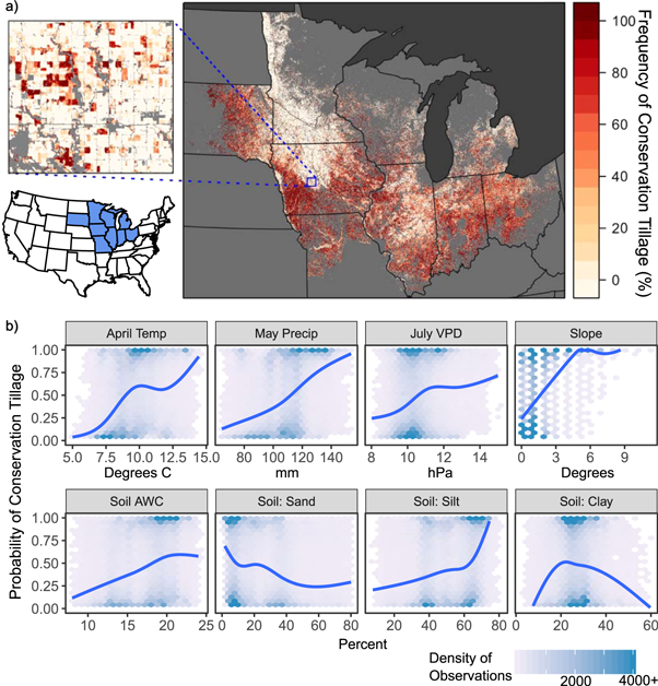
Figure 1. Satellite-derived tillage practices in the study area and environmental factors associated with long-term conservation tillage. (a) Study area inset and map of tillage frequency between 2005 and 2016. Tillage frequency was derived from 30 m Landsat data and is reproduced from Azzari et al 2019 [35]. Zoomed inset demonstrates variability on the landscape even in areas with a dominate tillage type. (b) Conditional probabilities of conservation tillage by environmental covariables from treatment propensity model. Estimates from individual field observations were smoothed with a GAM (blue line), and the density of field observations is indicated with blue shading. AWC = available water content; VPD = vapor pressure deficit.
Download figure:
Standard image High-resolution image2.2. Satellite-derived data sources
We used a previously published gridded dataset of annual tillage practices for the north central US from 2005 to 2016 by Azzari et al [35] to identify locations practicing conservation or conventional tillage at 30 m resolution (figure 1(a)). Briefly, these maps were generated by applying a random forest classifier trained on ground truth data from 5866 soybean fields to Landsat satellite imagery. Because the ground truth data was limited to soybean fields, the classification was applied only to pixels identified as soybeans based on annual crop type maps from the US National Agricultural Statistics Service (NASS) [45]. These soybean-based tillage maps achieve fairly complete coverage of the study region every two years due to dominant maize-soybean rotations. Here, we assume that the same tillage method was practiced during subsequent maize years. It is likely this assumption is not universally valid, since partial adoption characterizes over half of conservation tillage practitioners, with approximately 11% of farmers in this region adopting tillage practices by crop type [46]. Similarly challenging for inference, this product has an overall accuracy of 79%, with 84% and 72% of validation points correctly classified for conservation and conventional tillage, respectively. We mitigate these potential sources of error through additional data filtering criteria (section 2.3) and note that, given our findings (section 3.2), the possible inclusion of a small percentage of misclassified maize fields implies that our estimates of yield differences between conservation and conventional tillage systems are likely conservative.
Previously published yield maps for maize and soybean were produced using the Scalable Crop Yield Mapper (SCYM) [33], a satellite-based approach with a demonstrated ability to detect impacts from management practices [47, 48]. This approach has two main steps. First, statistical models predicting yields from crop phenology and climate covariates are derived from regionally parameterized crop models. Second, these statistical models are applied to satellite imagery and gridded climate datasets based on crop type maps, generating a yield estimate for each pixel. Maize yield maps were produced with Landsat satellite imagery for nine Corn Belt states from 2008 to 2015 by Jin et al [34]. We used the algorithm described therein to extend maize yield maps through 2017, with overall county-level agreement at r2 = 0.78 (RMSE = 1.2 t/ha) compared with NASS statistics. Soybean yield maps were produced by Lobell and Azzari [36] for the states of Indiana, Illinois, and Iowa from 2000 to 2015 with similar agreement to county yield statistics (r2 = 0.74, RMSE = 0.16 t/ha). Figure S1 (figure S1 is available online at stacks.iop.org/ERL/14/124038/mmedia) shows mean yields across space for each crop during the study period.
2.3. Field sample generation and covariate sampling
As noted above, the tillage map classification performs moderately well but contains some errors that could add noise to our analyses. To guard against spurious classifications, we restricted the tillage maps in the following ways: (1) we required pixels to have 6 observations during the 12 year dataset, with at least one observation before 2008 and after 2014, to ensure a dense time series of observations spanning the data record; (2) from these, we identified long-term tillage management regimes based on pixels with constant tillage status in all observations, indicating at least a decade of conservation practices and likely increasing the probability of sustained adoption in maize years; (3) we identified 'single-switch' pixels which switched tillage status one time between 2009 and 2014 to examine the impact of new tillage regimes; and (4) pixels needed to be part of a coherent pixel group of the same tillage classification and, for single-switch pixels, the same year (see Text S1). All remaining sampling and analyses occurred at this 'field entity' level. We then used a data-driven delineation of climate-soil domains [26] to sample up to 500 fields per tillage status within each domain for each year, resulting in 144 127 and 117 757 maize field-years and 92 037 and 100 222 soybean fields-years for conventional and conservation tillage, respectively.
For each field, we extracted the median yield from SCYM maps. We removed fields with outlier yield values below the 0.01% and above the 99.99% from both maize and soybean datasets. We then extracted median field values for a suite of environmental covariables defining both static field properties and annually varying weather and soil moisture. For static field properties, we obtained 1981–2010 climate normals from PRISM [49, 50], calculated field slope from the USGS National Elevation Dataset [51], and extracted soil properties for the top one meter from the SSURGO soil database [52]. Annual monthly and seasonal weather summaries were extracted from GRIDMET ∼4 km meteorological dataset [53]. Annual monthly modeled soil moisture and climate water deficit were extracted from the TerraClimate ∼4 km climatic water balance dataset [54]. Table S1 provides a list of all variables considered and their data sources. All data were accessed and processed in Google Earth Engine [55] with the exception of the soil data, which we acquired through SSURGO.
2.4. Analysis with machine-learning based causal inference
To quantify conservation tillage's impact on crop yields, we used causal forests, an recent adaptation of the classic random forest algorithm [56] for statistical inference on causal effects, particularly when heterogeneity is present [38, 39]. Broadly, causal forests act as an adaptive kernel method [39]; in our application, it uses each field's closest neighbors in covariate space to generate a counterfactual yield estimate under the alternative tillage practice. Causal forests generate mathematically valid confidence intervals while leveraging the ability of random forests to handle many covariates and nonlinear interactions without overfitting or requiring explicit model specification [38, 39, 57, 58]. Recent applications demonstrate better performance than conventional econometric methods for detecting and quantifying heterogenous treatment effects [59, 60].
Causal forests are also designed for observational datasets. Because treatments are not randomly assigned, an observational analysis could be confounded if fields that have higher (or lower) yields also tend to adopt conservation tillage at higher rates. Causal forests addresses these biases with a 'doubly robust' treatment estimation method (augmented inverse-propensity weighted estimation [61]) which combines both treatment propensity weighting [62] and regression adjustment to reduce sensitivity to misspecification in either model [39, 63].
2.4.1. Analysis of long-term conservation tillage
Here, we used the 'grf' package [64] in R [65] to implement causal forests separately for maize and soybean fields with long-term tillage practices (section 2.3). We designated 'conservation tillage' as the treatment variable, 'conventional tillage' as the control, and crop yield as the outcome. First, we used the full set of static covariates describing field slope, soil properties, and climate normals (tables 1 and 2) to estimate treatment propensity using 2000 trees and default function settings. The propensity model performed well, indicated by close agreement between propensity scores versus treatment status (figure S3). To examine biophysical factors typically associated with conservation tillage, we used the larger 9-state maize domain. We inferred variable importance from the number of times each covariate was used to split the individual trees, although it should be noted that correlations among variables can skew these metrics [66].
Table 1. Variables used in causal forests analysis: Maize. Variables are ordered by the proportion of splits on each variable within the ensemble of decision trees that make up each forest (high to low), which provides a rough approximation of variable importance. VPD = vapor pressure deficit; AWC = available water content. Table S1 provides data source information.
| Treatment propensity (30 yr climate normals) | Regression adustment/Expected yield outcome | Treatment effect |
|---|---|---|
| Slope | July mean max temp | Slope |
| May precip | May mean max temp | Soil clay content |
| April mean temp | Year | Soil sand content |
| April precip | July climate water deficit | June precip |
| July VPD | Solar radiation (June–August) | April soil moisture |
| June precip | August mean max temp | May mean min temp |
| July precip | May mean min temp | Early season precip |
| June VPD | June precip | August soil moisture |
| Soil sand content | Early season precip | Soil AWC |
| June mean temp | August soil moisture | June mean min temp |
| Soil silt content | June mean min temp | May mean max temp |
| Soil AWC | Growing Degree Days | June climate water deficit |
| May mean temp | May precip | July VPD |
| August mean temp | July precip | July mean max temp |
| July mean temp | August mean min temp | May precip |
| Soil clay content | Soil clay content | Growing Degree Days |
| Soil ksat | Soil AWC | April precip |
| Soil sand content | Solar radiation (June–August) | |
| August mean min temp | ||
| August mean max temp | ||
| July precip | ||
| April mean temperature | ||
| July climate water deficit | ||
| Year |
To meet the assumption of overlap within the causal forests framework, which requires that treatment and control samples occupy similar covariate space to provide appropriate neighbors for comparison, we then removed samples with propensity scores below 0.05 or above 0.95. This produced a final dataset of 70 404 and 88 220 (maize) and 51 215 and 68 334 (soybeans) unique field-year observations for conservation and conventional tillage, respectively. Figures S4 and S5 provide the spatial distribution of field observations before and after this propensity filter. We then specified the regression adjustment portion of the doubly robust estimator (see Text S2 and figure S2). Next, we used all covariables selected for this regression model and the most important variables in the propensity model (tables 1 and 2) to estimate the treatment effects of conservation tillage using the 'causal_forest' function in grf with 2000 trees and default parameters.
Table 2. Variables used in causal forests analysis: Soybeans. Variables are ordered by the proportion of splits on each variable within the ensemble of decision trees that make up each forest (high to low), which provides a rough approximation of variable importance. VPD = vapor pressure deficit; AWC = available water content. Table S1 provides data source information.
| Treatment propensity (30 yr climate normals) | Regression adjustment/Expected yield outcome | Treatment effect |
|---|---|---|
| Slope | Aridity (June–August) | May soil moisture |
| May precip | Previously Soy | April soil moisture |
| April mean temp | July climate water deficit | Slope |
| Soil silt content | Solar radiation (June–August) | July soil moisture |
| June VPD | June precip | Soil silt content |
| April precip | Growing Degree Days | July precip |
| Soil clay content | May soil moistre | Aridity (June–August) |
| July precip | June climate water deficit | Soil clay content |
| June precip | May precip | Soil sand content |
| May mean temp | Jan–April precipitation | June precip |
| August mean temp | July precip | August mean min temp |
| July mean temp | July soil moisture | Growing Degree Days |
| Soil AWC | Soil sand content | Soil AWC |
| June mean temp | April precip | July VPD |
| July VPD | June–August precip | Early season precip |
| Soil sand content | Soil clay content | Solar radiation (June–August) |
| Soil ksat | August mean min temp | April mean temp |
| Year | May precip | |
| Growing season precip | ||
| Previously Soy | ||
| April precip | ||
| June mean min temp | ||
| Year | ||
| June climate water deficit | ||
| July climate water deficit |
To investigate heterogeneity in treatment effects, we first tested for significant heterogeneity using the 'test_calibration' function in grf. We then summarized covariate values for subpopulations of observations based on their predicted treatment effects. Figures 2(a) and 3(a) show the distribution of field samples among these subpopulation bins. We then identified covariates with stronger influences on the yield outcomes of conservation tillage based on covariate distributions within these subpopulations and informed by variable importance rankings for the causal forests (tables 1 and 2).
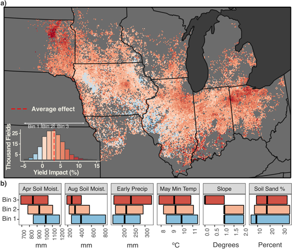
Figure 2. Distribution of maize yield impacts from conservation tillage from 2008 to 2017. (a) Mean conditional treatment effect for all field-year observations on a regular 5 km2 grid. The distribution of treatment effects across all 158, 624 field observations is provided in the histogram, with indicators for subpopulation bins used to analyze heterogenous treatment effects across covariates. (b) Covariate distributions (median + interquartile range) by treatment effect subpopulation bins for variables influencing heterogenous impacts on the landscape.
Download figure:
Standard image High-resolution image2.4.2. Analysis of fields following initial tillage conversion
To assess the initial yield impacts from switching tillage practices, we applied the same causal forests approach to the fields we identified as 'single-switch' fields (section 2.3). We conducted one cross-sectional analysis for the final year of yield data for each crop (2017 for maize and 2015 for soybeans) to evaluate the partial treatment effect of each additional year of conservation tillage. Here, the treatment variable was the number of years since adoption, with zero indicating the control case of continued conventional tillage. We then conducted the same analysis on fields that switched from conservation tillage to conventional tillage. We note that the location of fields switching to and from conservation tillage are not similarly distributed in space (see figures S6 and S7), so the spatial support for these analyses is not directly analogous to one another.
2.4.3. Confounders and omitted variables
Socioeconomic factors for which we lacked data can influence adoption, and, if also associated with higher yields, they could cause omitted variable bias in our propensity score and treatment effect estimation. For example, farm size, education, high sales farms, and regulations for highly erodible lands have been positively correlated to conservation tillage adoption [18, 32, 67–70]. Negative correlations exist for farmer age, management by renters, and distance from research stations [32, 68, 69]. Because lower intensity tillage reduces fuel requirements, high fuel costs can also promote adoption [70]. Still, it remains difficult to predict adoption due to a lack of universal features [71, 72], suggesting there is variability in these effects. Nevertheless, the propensity model we developed based upon biophysical factors captures the probability of adoption well (figure S3), and causal forests's doubly robust estimator buffers some misspecification in the propensity score model (section 2.4). Future large-scale randomized experiments or quasi-natural experiments able to collect data on these attributes would be a useful robustness check for the analysis.
3. Results and discussion
3.1. Biophysical factors associated with conservation tillage
Overall, we found that long-term conservation tillage occurred across a wide range of environmental conditions, as indicated by treatment probabilities above 25% across most covariable values (figure 1(b)). This is consistent with past difficulties identifying universal variables to explain adoption [71, 72]. Field slope ranked highest in importance (table 1), likely explained by greater benefits for erosion relative to flatter fields and policies targeting highly erodible areas [18]. Higher early season temperature, early season precipitation, and July vapor pressure deficits also increased probability of adoption (figure 1(b), table 1), consistent with findings that conservation tillage is often more prominent in warmer, arid conditions [16, 17, 73] and can enhance water infiltration rates [1]. Both soil silt and available water content were positively related to conservation tillage while sand content was negatively correlated (figure 1(b)), although soil variables did not rank high in variable importance.
3.2. Yield effects of long-term conservation tillage
For maize, we found an overall 3.3% yield benefit from conservation tillage (average treatment effect; 95% Confidence Interval, CI = [3.1%, 3.4%]) across fields with long-term tillage practices from 2008 to 2017. This translated to an average yield boost of 0.36 t/ha (CI = [0.34, 0.37]). For soybeans, we found a smaller yield benefit of 0.74% (CI = 0.53%, 0.95%) or 0.024 t/ha (CI = 0.017, 0.031) from 2005 to 2015 within Indiana, Illinois, and Iowa. Generally, these effects are smaller than typical year-to-year yield variability in this region (figure S2) and similar in magnitude to previous plot level work [20, 21, 27, 74, 75]. We did, however, find more evidence for positive yield impacts across the region than the majority of existing literature [16]. This may reflect ongoing technology improvements for conservation tillage implementation [29] or additional insight afforded through our methodology, which allows the inclusion of a large range of covariates and leverages thousands of fields across a wide region.
Tests for treatment effect heterogeneity were significant for both maize (p < 0.0001) and soybeans (p < 0.0001), indicating treatment effects are moderated by the weather, soil, and slope covariates used. For maize, the 5th–95th percentiles of these conditional average treatment effects (CATEs) ranged from −1.3% to 8.1%; for soybeans, they ranged from −4.7% to 5.8%.

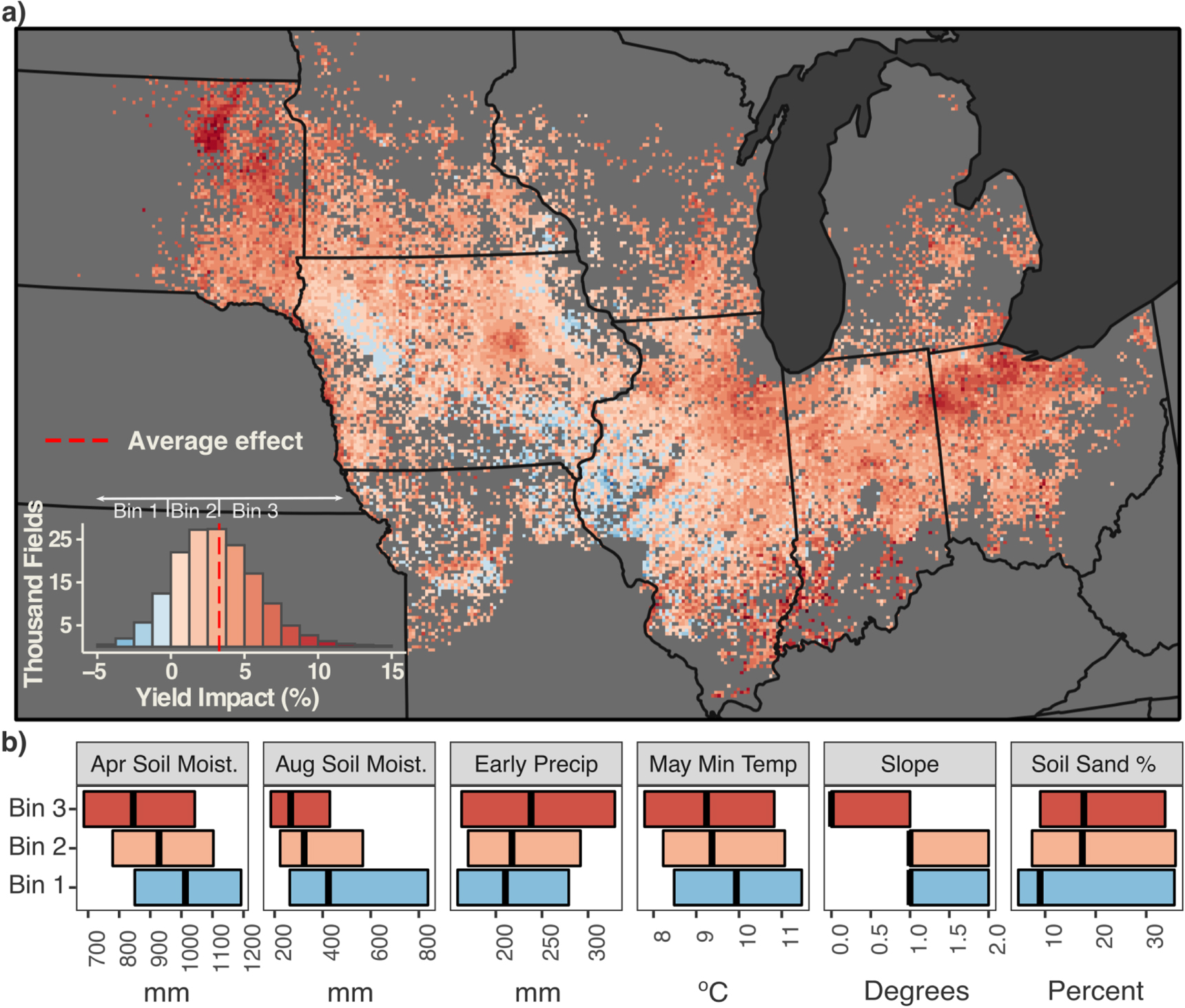
Figure 3. Distribution of soybean yield impacts from conservation tillage from 2005 to 2015. (a) Mean conditional treatment effect for all field-year observations on a regular 5 km2 grid. The distribution of treatment effects across all 119, 549 field observations is provided in the histogram, with indicators for subpopulation bins used to analyze heterogenous treatment effects across covariates. (b) Covariate distributions (median + interquartile range) by treatment effect subpopulation bins for variables influencing heterogenous impacts on the landscape. AWC = available water content.
Download figure:
Standard image High-resolution imageTo understand how this heterogeneity manifested across the Corn Belt, we mapped the mean CATE for all field-years on a 5 km2 regular grid by crop type (figures 2(a) and 3(a)). For both maize and soybeans, negative impacts from conservation tillage were most pronounced in northwestern Iowa and from southeast Iowa into western Illinois. Conservation tillage largely improved yields from eastern Illinois through Indiana. For maize, Ohio, South Dakota, and the outer regions of the Corn Belt displayed strong positive effects. Notably, we found that conservation tillage had a largely positive effect on maize yields in the northern Corn Belt, where it has historically been more limited in practice (figure 1(a)). While it is possible this effect is driven by early adopters inordinately adept at managing their fields, recent studies in Minnesota [29, 76], New York [12], and Canada [32] provide increasing evidence for conservation tillage interest and feasibility in these more northerly latitudes.
3.3. Soils and annual weather moderate yield impact
To understand the underlying biophysical features driving these patterns, we explored conditional treatment effects by field attributes for both maize (figure 2(b)) and soybeans (figure 3(b)). Overall, the soil water balance and seasonal temperatures seem to drive much of the heterogeneity observed. For example, maize and soybean yield benefits were greater than average when baseline late-season (July–August) soil moisture was low, suggesting higher differential success in arid conditions likely due to improved soil water holding capacity. Similarly, soybean field-years with positive yield effects tended to have lower baseline soil available water content from static soil maps, indicating potential improvement in water capacities on these fields from conservation tillage.
In addition to these arid conditions generally thought to benefit from conservation tillage [16], we also found evidence that conservation tillage can improve yields under wet conditions. Soybean field-years with positive yield impacts had higher median July precipitation (figure 3(b)). Similarly, maize field-years with the greatest treatment effects experienced higher median early season precipitation (figure 2(b)). Together, this suggests improved water infiltration on fields under conservation tillage.
On the other hand, we also found evidence that very wet early season soils (April–May) can reduce conservation tillage benefits in both crops. Conventional tillage helps dry water-logged soils [77], often enabling earlier planting dates and thus better yields. Interestingly, conservation tillage performed worse for maize when mean May minimum temperature was higher (figure 2(b)). Although higher temperatures should help dry soils near planting, higher May temperatures could also facilitate weed growth that can compete with maize emergence or, combined with residue cover, increase disease pressure by fostering disease organisms.
Although higher field slopes increased the likelihood of conservation tillage (figure 1(b)), yields were not better on higher slopes for either crop (figures 2(b), 3(b)), possibly because impacts from soil erosion operate on centennial time scales not yet manifested here. However, we were unable to compare fields with slopes higher than 3 degrees due to lack of overlap between tillage types, since high sloped fields had high probabilities of treatment (figures 1(b), section 2.4.1).
3.4. Initial yield impacts from switching tillage practices
There is strong evidence that any benefits from conservation tillage can be absent upon initial implementation and accrue over time as soil health and management improves [16]. For maize and soybeans, we found an overall positive yield effect of 0.29% and 0.033%, respectively, for each additional year under conservation tillage when considering fields between 1 and 8 years since adoption. Although still positive, these effects are an order of magnitude smaller than fields with long-term conservation tillage (figure 4). These numbers imply that, on average, the full yield benefit of long-term conservation tillage is achieved after 11 years for maize and 22 years for soybeans. Interestingly, we found similar (maize) or greater (soybeans) yield improvements when analyzing fields that switched from conservation tillage to conventional tillage (maize: 0.26%; soy: 0.61%). This suggests that management challenges persist for conservation tillage, likely related to weed control or timing of planting. Indeed, a previous analysis found that in the US circa 2012, less than half of farmers reporting 'no-till' methods practiced them continuously during the previous four years [18]. Because soil benefits are greatest under sustained conservation tillage, there is still a need for improved understanding of these management decisions and challenges.

Figure 4. Summary of the average yield impacts of conservation tillage by implementation duration. Dark bars represent long-term tillage management in fields that had consistent tillage classification from 2005 to 2016. Light bars represent fields which switched to conservation tillage during this study period, with years since conversion ranging from 1 to 8. Error bars denote 95% confidence intervals.
Download figure:
Standard image High-resolution image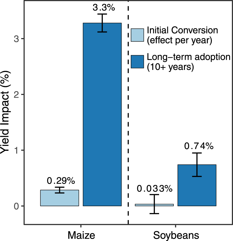
4. Conclusions
By applying causal inference methods to Earth observation datasets, we found that long-term conservation tillage typically has a small positive yield effect for both maize and soybeans across tens of thousands of fields in the US Corn Belt. This effect is diminished on fields that recently switched from conventional to conservation tillage, supporting the notion that it can take several years to achieve yield benefits due to a time lag in soil response and the learning curve for effective management [16]. Compared with background yield variability from annual weather patterns, cultivars, and management practices in this system, these yield effects are small and would be difficult to detect with localized experiments on small sample sizes. Our satellite-based approach allows us to pool the experience of over 150 000 field observations, improving the ability to detect this signal amid other variation.
Given these rare or minor yield penalties, our results support an emerging consensus that tillage adoption decisions can focus on factors other than yields in this region [20, 75]. In addition to positive effects on soil quality, conservation tillage is typically associated with lower production costs due to reduced machinery, fuel, and labor requirements [1, 24, 78]. Conservation tillage can also reduce supplemental water requirements [27] and field fallowing frequency, enabling increased crop production over time [78]. These savings often counterbalance yield penalties in more marginal areas [27]. In other cases, conservation tillage can have unclear or negative effects. Improved soil carbon storage and reduced NO2 emissions are sometimes heralded as a benefit of conservation tillage, but study findings are mixed [4, 16, 28, 30]. Similarly, although conservation tillage can reduce surface runoff, accumulated P in the soil can result in high P runoff during storm events that impacts downstream water quality [79]. Ultimately, conservation tillage systems reduce soil erosion, often returning soil loss rates to background levels on par with natural soil generation [2].
Our assessment compares on-the-ground, production-scale fields at a systems level. It is generally understood that a suite of management changes are associated with reduced tillage. We provide evidence that conservation tillage systems are capable of achieving modest yield improvements, but we are unable to attribute yield gains to specific components of any management regime. For this reason, complementary large-scale or quasi-natural experiments with detailed management data would be useful to characterize best management practices. Our results support soil conservation practices by demonstrating that conservation tillage can be used with minimal and typically positive yield impacts under what are likely a set of optimized management practices.
Acknowledgments
We thank Xinkun Nie for guidance on analyses, Brian Lin for retrieval of statistics from the US agricultural census and Anthony Kendall for assistance with soil data processing. Funding was provided by the NASA Harvest Consortium grant 54308-Z6059203 to DBL. Any opinions, findings, and conclusions or recommendations expressed in this material are those of the authors and do not necessarily reflect the views of NASA.
Data availability statement
Data and code necessary to support the findings of this study and reproduce the analyses and figures is available at https://doi.org/10.5281/zenodo.3525346 and https://doi.org/10.5281/zenodo.3525359, respectively. This includes the field-level samples derived from the annual tillage and yield map datasets, along with associated covariates. Due to privacy concerns, field locations are reported by county only (latitude and longitude have been removed), and the input map datasets are not publicly available.