

Abstract
Climate change, urbanization, and economic growth are expected to drive increases in the installation of new air conditioners, as well as increases in utilization of existing air conditioning (AC) units, in the coming decades. This growth will provide challenges for a diversity of stakeholders, from grid operators charged with maintaining a reliable and cost-effective power system, to low-income communities that may struggle to afford increased electricity costs. Despite the importance of building a quantitative understanding of trends in existing and future AC usage, methods to estimate AC penetration with high spatial and temporal resolution are lacking. In this study we develop a new classification method to characterize AC penetration patterns with unprecedented spatiotemporal resolution (i.e. at the census tract level), using the Greater Los Angeles Area as a case study. The method utilizes smart meter data records from 180 476 households over two years, along with local ambient temperature records. When spatially aggregated, the overall AC penetration rate of the Greater Los Angeles Area is 69%, which is similar to values reported by previous studies. We believe this method can be applied to other regions of the world where household smart meter data are available.
Export citation and abstract BibTeX RIS
1. Introduction
Globally, the use of air conditioning (AC) is expected to increase significantly over the coming decades, particularly across the developing world. Although 87% of US households currently have air conditioners (ACs), the US still led the world in new sales of ACs in terms of cooling output capacity (about 315 GW) in 2016 (International Energy Agency/Organisation for Economic Co-operation and Development 2018). Worldwide, AC penetration is estimated to grow dramatically from 1.6 billion units currently to 5.6 billion units by mid-century (Pierre-Louis 2018), most of which will be driven by developing countries like China, India, and Indonesia. Furthermore, future increases in daily average ambient temperatures and more frequent extreme heat waves resulting from global climate change will increase the usage of current AC installations (Auffhammer et al 2017). Thus, global AC growth will reflect both increases in adoption (Bartos et al 2016) and increases in the use of existing AC capacity. This growth can exacerbate warming at both global (i.e. from increased greenhouse gas emissions) and urban scales (i.e. from increased anthropogenic heat (Wang et al 2018)), resulting in a positive feedback loop that accelerates the need for more cooling.
Despite the importance and urgency of understanding future trends in AC growth, current research quantifying AC penetration with high spatial and temporal resolution is lacking. Estimating AC penetration rates with high spatial resolution would be particularly valuable for identifying communities that might be vulnerable to extreme heat events due to the lack of AC or rising energy costs. Developing knowledge of these AC penetration patterns would also be useful for future grid planning, as it would enable the identification of peak energy hotspots, as well as areas that might be prone to large increases in AC installations in the future. Developing an understanding of the temporal changes in AC penetration rates is also important, particularly in areas where AC usage is currently low and its growth potential is high.
Past studies estimate AC penetration rates at low spatial resolution due to a lack of available data. Most reported AC penetration rates come from appliance saturation surveys or residential energy consumption surveys carried out by federal and state governments, which are often time-intensive undertakings (e.g. multi-year efforts) (Palmgren et al 2010) and constrained by budgets (Witt et al 2017). The spatial resolutions of existing datasets typically range from climate zones (e.g. in the case of California (Lutzenhiser et al 2016), which tends to have more available data than other regions of the US) to larger geographic regions (e.g. groups of multiple states (US Energy Information Administration 2018a)). The latest 2015 Residential Energy Consumption Survey (RECS) released by the US Energy Information Administration in 2018 showed that the Pacific region (comprised of Alaska, California, Hawaii, Oregon, and Washington) of the US had an overall AC penetration rate of 66% (US Energy Information Administration 2018b). In California, the Advanced Residential Energy and Behavior Analysis Project conducted by the California Energy Commission (CEC) revealed that over 60% of all California homes had AC units (Lutzenhiser et al 2016). More detailed data at the utility level were reported through the 2009 California Residential Appliance Saturation Study, which indicated that 75% of customers in the Southern California Edison utility territory had AC equipment in 2009 (Palmgren et al 2010). These reports have major shortcomings because of the long time between updates and their low spatial resolution. Other studies (e.g. McNeil and Letschert 2008, 2010, Sasaki et al 2015) have used economic and demographic parameters to model the diffusion of residential appliances including AC, but these studies have only achieved results at the country-scale (i.e. they report one value for entire countries). New methods are needed to derive higher resolution estimates of AC penetration rates to facilitate better planning from an energy management perspective.
Smart meter data have enabled a diversity of analyses in the building energy space. A subset of these analyses, which include peer-reviewed studies (Fels 1986, Kreider and Haberl 1994, Haberl and Kreider 1994, Kissock et al 2003, Ali et al 2011, Pampuri et al 2016, Gouveia et al 2017, Perez et al 2017) and open source platforms (Borgeson 2016, OpenEE Inc. 2018), estimate cooling and/or heating loads from whole building energy consumption data. Other analyses have used smart meter data to calculate potential energy savings from demand response (DR) programs (Kwac and Rajagopal 2013, Dyson et al 2014, Borgeson et al 2015) and disaggregate energy consumption according to end-use activity from whole-building data (Froehlich et al 2010, Kolter et al 2010, Zeifman and Roth 2011, Carrie Armel et al 2013). (While methods have been established to disaggregate the electricity consumption signatures of individual appliances (e.g. an AC unit) (Froehlich et al 2010, Kolter et al 2010, Zeifman and Roth 2011, Carrie Armel et al 2013), they typically require data at the minute-level resolution or higher, which is higher resolution than is supported by most smart meter infrastructure (Borgeson 2013). Despite the growing body of literature utilizing these datasets, studies that use smart meter data for determining highly-resolved AC penetration rates are lacking.
In this study we present a new method to compute AC penetration rates with high spatial resolution (i.e. the census tract level) utilizing the electricity consumption records of 180 476 households in the Greater Los Angeles Area along with local site weather data. Our proposed method is capable of differentiating households that currently use space cooling from those that do not. Trends in AC penetration are then analyzed in the context of regional variations in climate. Given that only 65% of homes in the western US currently have AC (compared to 95% in the South (US Energy Information Administration 2018b)), future increases in AC use in the US are likely to expand in the West, particularly in dense regions such as Los Angeles that are growing in population and will experience increasing temperatures (Sun et al 2015, Walton et al 2015). Moreover, Los Angeles is diverse in terms of its socioeconomic demographics, enabling us to observe differences in AC penetration across disparate groups. Furthermore, the Greater Los Angeles Area is observed and projected to have uneven spatial distributions of warming due to urban heat islands and future climate change, respectively (Hall et al 2012, Sun et al 2015, Walton et al 2015, Vahmani et al 2016, Li et al 2019). Hence, the Los Angeles region represents an important area to assess AC penetration rates at high spatiotemporal resolution. Such knowledge can help enable (a) tracking AC adoption over time and (b) projecting the spatiotemporal trends in future AC growth, which is important for managing peak energy demand, guiding electricity asset investments, and building energy efficiency and demand-side management incentives. There is also an abundance of available smart-meter data in the Greater Los Angeles Area, enabling analysis with unprecedented spatiotemporal resolution.
2. Methods
2.1. Datasets
We obtained hourly residential electricity data records from the Investor Owned Utility (IOU), Southern California Edison, for the years 2015 and 2016. The dataset contains more than 200000 randomly chosen households across the Greater Los Angeles Area. The sample size of 200000 was calculated to be representative of the region's 4.5 million residential households at a 99% confidence level. We screened out customers that had less than an entire year of electricity records. We also did not consider homes that were mostly uninhabited, determined as those whose annual electricity consumption was lower than 20 kWh, which is the amount of electricity an average home in California consumes per day (Energy Information Agency 2009). Although no information about onsite generation installation (e.g. solar panels) was provided by the utility, a heuristic filtering approach was applied to remove homes with solar generation to avoid distorting electricity–temperature relationships. Customers who had no electricity consumption for at least one hour between 10:00 and 16:00 and positive electricity consumption between 17:00 and 23:00 for more than 36 d (5% time of the 2 year span) were considered to have solar generation. Although this method would be insufficient to detect homes that had enough battery storage to offset night-time electricity generation, we expect these instances to be very small in number. (Note that zeros, rather than negative values for electricity use, were reported in the dataset for hours when self-generation exceeded consumption.) After all filtering was complete, 180 476 households were included for analysis in this study (see statistics of analyzed data records in table S1). Household street addresses were also provided to enable geospatial analysis. All data were stored and processed on USC's Center for High-Performance Computing (HPC) with a highly secure HPC Secure Data Account, allowing us to perform computations that met the strict data security requirements of the IOU.
Two sources were used to retrieve daily average ambient near-surface air temperature (hereafter referred to as 'daily average ambient temperature') data for the years under investigation (2015 and 2016): the California Irrigation Management Information System (CIMIS) and the National Oceanic and Atmospheric Administration's National Centers for Environmental Information (NCEI). Both networks are made up of land-based, automated, quality-controlled weather stations that cover most population centers in Southern California. This study utilizes 36 CIMIS stations and 43 NCEI stations, which were selected from all available stations by choosing the nearest weather monitors to each household with electricity data records.
Census tract boundary shapefiles were acquired from the US Census Bureau website (US Census Bureau 2017). Building climate zone boundaries established by CEC, based on building energy consumption characteristics, were also retrieved to characterize climate in the investigated region (California Energy Commission 2015). Sample records that fell within each census tract were counted and compared against the sample sizes needed to statistically represent the population of that census tract. Detailed methods can be found in the supporting information (available online at stacks.iop.org/ERL/14/094004/mmedia).
2.2. Statistical model
To describe the nonlinear relationship between residential electricity consumption and ambient temperature, we implemented the segmented linear regression model described in our previous study (Chen et al 2018). In this model, a stationary point is located by iteration to achieve the overall best two-piece linear fit to the dataset. Our previous study (Chen et al 2018) shows that using daily accumulated electricity consumption data and daily mean temperature yields the best model performance. Hence, we aggregated hourly electricity data records to daily accumulated electricity consumption (kWh day−1) for analysis. Three examples of this segmented model showing daily electricity consumption versus daily average ambient temperature for households in the Greater Los Angeles Area are illustrated in figure 1.
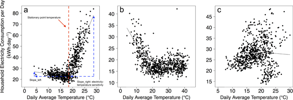
Figure 1. Daily cumulative electricity consumption versus daily average ambient temperature for three example homes in the Greater Los Angeles Area. Stationary point temperature (SPT), electricity–temperature sensitivity (i.e. the slope of the least squares best fit for temperature values ≥ SPT, labeled as 'slope_right'), and the slope for temperature values < SPT (labeled as 'slope_left') are identified in panel (a). Panel (a) illustrates a home identified by our method as having AC, whereas (b) and (c) are identified as not having AC.
Download figure:
Standard image High-resolution imageTwo physically-relevant metrics can be retrieved from the segmented linear regression: (1) the stationary point temperature (SPT), which represents the stationary point identified by the regression model, corresponding to the threshold ambient temperature beyond which households are likely to use AC (see distribution of SPT in figure S3, and (2) electricity–temperature sensitivity (E–T sensitivity), the slope of the least squares linear regression for temperature values ≥ SPT (figure 1(a)). Physically, this metric represents the change in electricity consumption for a household corresponding to a unit increase in ambient temperature.
To determine whether a household has AC, our method compares the slopes of least squares regressions for temperature values falling below SPT (referred to as slope_left) versus that for temperature values greater than or equal to SPT (referred to as slope_right) (see figure 1(a)). We define households with AC as those that meet both of the following criteria: (1) slope_right greater than zero, and (2) the sum of slope_left and slope_right greater than zero.
Electricity consumption versus temperature for a typical household with AC is shown in figure 1(a). In this case, electricity consumption increases when the daily average ambient temperature is greater than or equal to SPT, presumably due to increased cooling demand, thus meeting criteria (1). Criteria (2) is set mainly to rule out households that have negligible positive slope_right caused by noise or other appliances that might consume more electricity on hot days like refrigerators (Saidur et al 2002); it removes the need to set an arbitrary non-zero cut-off value for slope_right to account for a possible positive but negligible slope_right. According to data from the 2015 Residential Energy Consumption Survey, space heating in Southern California is mainly supported by natural gas, and thus, would not impact analysis of electricity–temperature sensitivity (US Energy Information Administration 2017); meanwhile, households in the investigated region generally consume more electricity for space cooling than heating (California Energy Commission 2014). Hence, slope_left is typically near-zero, with an absolute value much less than slope_right. (See supporting information figure S2 showing slope_right versus slope_left values).
Households that do not meet the two criteria above are deemed as having no AC. Electricity consumption versus temperature for two example households identified as having no AC are shown in figure 1(b) and 1(c). The household in 1(b) does not fulfill the condition slope_left + slope_right > 0, while that shown in 1(c) does not fulfill the condition slope_right > 0. Visually we see no significant energy use increase, even on hot days when daily average ambient temperature exceeds 30 °C (86 °F), suggesting no AC usage.
It is important to note that these criteria may not be sufficient to identify AC penetration in all regions throughout the US and rest of the world. Applicability to other locations is discussed in the discussion section. For more discussion about shortcomings of this method, please see the Supporting Information section S2.
We applied this classification framework to partition the full dataset (180 476 households) into two categories, i.e. households with and without AC, for the two years investigated. We then computed AC penetration rates, discussed below in section 3.1, at the census tract level by dividing the number of households identified as having ACs by the number of households in our dataset falling within each respective census tract.
3. Results and discussion
3.1. AC penetration rates
One of the major advantages of the method proposed in this study is the ability to quantify AC penetration rates at high spatial resolution. Figure 2 displays the spatial distribution of AC penetration rates in the Greater Los Angeles Area at the census tract level. Since our source data was provided by Southern California Edison, penetration rates are not shown for regions served by other utilities (e.g. Los Angeles Department of Water and Power). Census tracts containing too few records to statistically represent the population are designated with cross-hatching. (Note that the entire dataset is representative of the overall population at a 99% Confidence level, while the data shown at the census tract level in figure 2 are representative at the 90% Confidence level, except where noted with cross-hatching.)

Figure 2. A choropleth map of AC penetration rates (i.e. the ratio of total number of homes identified with AC versus the total number of homes per aggregation area in our dataset) for all census tracts in the Greater Los Angeles Area that are powered by Southern California Edison. Generally, coastal and mountainous areas tend to have lower AC penetration rates relative to inland and desert areas. The dark gray boundaries indicate building climate zones, with average summer temperatures per climate zone indicated at the bottom of the figure. White indicates that no data were available. Cross-hatched census tracts do not have sufficient records to statistically represent the population with a 90% confidence level and margin of error of 10%. These tracts account for 30% of analyzed census tracts.
Download figure:
Standard image High-resolution imageSince AC penetration rates are calculated using household level data, AC penetration rates can be estimated at any spatial resolution so long as the sample size per aggregation area is statistically representative of the region. For reasons of privacy protection, data were aggregated to the census tract level. (Census tracts, established by the US Census Bureau, are small and relatively stable geographical units in terms of area and population (US Census Bureau 2019)). To the authors' knowledge, this is the first peer-reviewed study to calculate AC penetration rates with high spatial resolution.
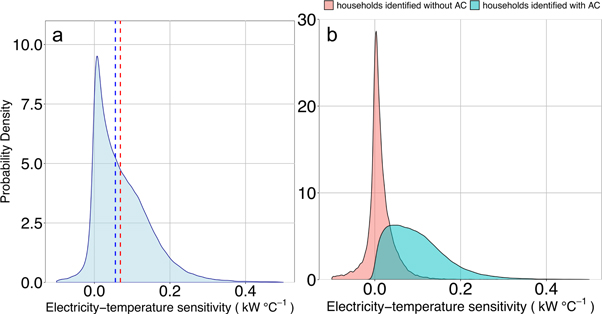
The overall AC penetration rate in the investigated area is computed as 69%. Figure 3 shows probability density distributions of electricity–temperature sensitivities for all households included in our dataset (figure 3(a)) and separately for homes classified with and without AC (figure 3(b)). The mean (median) electricity–temperature sensitivity for all households is 0.068 (0.054) kW °C−1 (figure 3(a)).
Figure 3. Probability density distributions of E–T sensitivities (a) for all 180 476 homes investigated in this study, and (b) shown separately for homes identified as having AC (in blue-green) and those identified as not having AC (in red). In (a), the red dashed line indicates the mean E–T sensitivity value (0.068 kW °C−1) for all homes, while the blue dashed line indicates the median (0.054 kW °C−1).
Download figure:
Standard image High-resolution image
Though there is some overlap between the probability density distributions for homes identified with and without AC, we see that most households with near-zero and negative sensitivities are grouped into those without AC, as we would expect. On the contrary, households with AC have a wider range of E–T sensitivities. One of the advantages of this classification method for determining whether or not a household has an AC unit is that there is no need to define an arbitrary cut-off based on electricity–temperature sensitivity. On the other hand, the lack of a 'cut-off' also results in the region overlap in E–T sensitivities between the two groups in figure 3(b).
Generally, AC penetration rates are higher in hotter climate zones (note the average summertime temperatures per climate zone indicated in figure 2). Along the coast, low AC penetration rates are observed, with the exception of a few census tracts that are generally in more wealthy regions (not shown). Compared to other locations within the study domain, coastal areas, which are mainly included in Climate Zone 6, have the lowest summer mean temperature, resulting in a relatively low demand for cooling. Climate Zone 16, spanning inland, mountainous regions, has lower AC penetration rates relative to surrounding areas on the east side of the basin, likely due to its relatively low summer mean temperature. Also, Climate Zone 16 includes Big Bear Lake, a resort area utilized for skiing and winter vacationing, leading to a portion of seasonal residents who may not install or use ACs. Future work can explore other causes of spatiotemporal variation in AC penetration rates, such as socioeconomic status and building characteristics.
3.2. Comparison of computed AC penetration rates to other studies
Here we compare aggregated AC penetration rates presented in this investigation to existing survey data for the studied region (table 1). The overall calculated AC penetration rate for all 180 476 households (69%) is slightly less than the California Residential Appliance Saturation Study value for the SCE territory (75%). It should be noted that our classification method might not identify evaporative cooling devices as they consume much less energy than central or room ACs (Maheshwari et al 2001), and therefore, are unlikely to cause a significant increase in electricity consumption per unit temperature increase when used. If we consider that the California Residential Appliance Saturation Study estimates that 6% of cooling systems in Southern California are evaporative, our results are consistent with its computed penetration rate.
Table 1. Comparison of AC penetration rates acquired from this study versus previous studies.
| Source | AC penetration rate | AC types included | Investigated year | Investigated area | Citation |
|---|---|---|---|---|---|
| This study | 69% | All types (other than possibly evaporative cooling devices) | 2015–2016 | Southern California Edison territory | |
| Residential Energy Consumption Survey | 66% | All types | 2015 | Pacific region of US | (US Energy Information Administration 2018b) |
| Advanced Residential Energy and Behavior Analysis Project | >60% | All types | not provided | California | (Lutzenhiser et al 2016) |
| California Residential Appliance Saturation Study | 75% | All types (including 6% evaporative coolers) | 2009 | Southern California Edison territory | (Palmgren et al 2010) |
| Borgeson PhD Dissertation | 60% or 68%–70%a | All types | 2008–2011 | Pacific Gas and Electric territory | (Borgeson 2013) |
A more recent report, the Advanced Residential Energy and Behavior Analysis Project, released by California Energy Commission, suggests that California's overall AC penetration rate is >60%, which is consistent with our value though is representative of a larger region. In his PhD dissertation, Borgeson (2013) calculated the AC penetration rate for Pacific Gas and Electric's territory in 2008 through 2011, which covers large portions of Northern and Central California, as 60% or 68%–70%, depending on which of two different methods was employed (Borgeson 2013).
3.3. Applicability to other regions
We believe that this method can be applied to other regions around the world where household level smart meter data are available. However, some modifications to the method might be required in some cases, depending on the region under investigation. Three factors should be taken into consideration to determine whether modifying the method is needed: climate characteristics (energy demand for space cooling and heating), the typical fuel(s) utilized for space cooling and heating, and most common AC and heating technologies utilized. These three factors together determine the quantitative relationships between household electricity consumption and ambient temperature.
Although US regions have diverse space cooling and heating needs (Sivak 2013) as well as fuel choices (US Energy Information Administration 2017), we expect the methods defined in this study to be applicable for much of the country under current climatic and fuel usage trends. For example, US regions with cold winters, including the east coast, the mid-west, and the west, typically use natural gas as the dominant space heating fuel (US Energy Information Administration 2017). Thus, we would not expect a strong electricity–temperature sensitivity on days when temperatures are cold enough to require heating, meeting the criteria to use the method defined in this study. In the Southern US, which typically has a hot-humid climate, electricity is the main space heating energy source during their mild and short winters (US Energy Information Administration 2017). Considering the intense use of AC in the summertime in hot-humid regions, even in this case slope_right would be anticipated to be larger than the absolute value of slope_left; thus, in these regions our method would likely be viable. This reasoning is supported by a study in Shanghai (Li et al 2018), which has a comparable hot-humid climate, significant use of electric heating, and similar AC penetration rate (near-100%) to the Southern US (US Energy Information Administration 2018b, Li et al 2018, Spark 2019). In this study, they find that cooling drives residential electricity usage when compared to heating, suggesting that our method could be effective even in warm regions where electric heating dominates.
The US is expected to electrify over time (Deason et al 2018). The 2015 RECS observes more electric heating in the residential sector than 2009 RECS (Energy Information Agency 2018). The methods presented here would likely need to be modified, for example, in cases where the change in energy usage per change in temperature during electric heating (i.e. slope_left) would exceed the rate of change during electric cooling (i.e. slope right). Our method might also fail in regions with year-round hot climates, such as those near the equator, as it might be difficult to identify a stationary point temperature in relationships between household electricity consumption and ambient temperature in cases where cooling is required all year. These households would likely have a linear positive slope in electricity–temperature plots without an identifiable stationary point.
Lastly, AC type should be checked, particularly in regions with high usage of evaporative cooling, since this cooling type requires less energy and is therefore more difficult to identify from electricity use records. Consequently, this method would likely be less effective in identifying evaporative cooling through the use of electricity–temperature plots.
Above all, such methods cannot be applied without an abundance of household level smart meter data, as well as reliable, high-resolution weather data.
To conclude, a new classification method to identify whether homes have AC at the household level was developed and presented here. The method relies on having access to household daily aggregated electricity and daily average ambient temperature data. The methods were applied to estimate AC penetration rates at the census tract level in the Greater Los Angeles Area (within the Southern California Edison service territory). The mean penetration rate computed for the service territory was also compared to estimates from previous studies. Using our study as a baseline for AC penetration, repeating the study in future years could allow for quantifying trends in AC penetration over time.
Acknowledgments
This work was funded in part by the Teh Fu 'Dave' Yen Fellowship in Environmental Engineering awarded to Mo Chen at University of Southern California. This work was also funded in part by the National Science Foundation under grants CBET-1512429, CAREER Grant CBET-1752522, EAGER-1632945 and CAREER Grant 1845931. Computation for the work described in this paper was supported by the University of Southern California's Center for High-Performance Computing (hpcc.usc.edu). We also thank Southern California Edison for access to the smart meter data.
Data availability statement
The data that support the findings of this study may be available from the corresponding author upon reasonable request. These include processed data used to create figures. The raw data are not publicly available for legal and/or ethical reasons.