Effects of global warming and solar geoengineering on precipitation seasonality

Prasanta Kumar Bal; Raju Pathak; Saroj Kanta Mishra; Sandeep Sahany

doi:10.1088/1748-9326/aafc7d

1. Introduction

As a result of climate change, precipitation increases are very likely in high latitudes, while decreases are likely in most of the tropics and subtropical land regions (Intergovernmental Panel on Climate Change (IPCC) 2007). Climate change not only affects annual precipitation accumulation but it also alters the precipitation distribution spatially and temporally (in terms of extreme precipitation, timing and length of the peak precipitation period; Min et al 2011, Collins et al 2013, Pascale et al 2015). The socio-economic conditions of many countries significantly depend on seasonal rainfall and its variability (Gadgil and Gadgil 2006). Any change in precipitation intensity, duration and timing of the peak precipitation period from their normal conditions, significantly influences agriculture, biodiversity and the overall ecosystems (Gadgil and Gadgil 2006, Nelson et al 2009, Feng et al 2013). Hence, the spatial and temporal distribution of precipitation and its likely changes under global warming are important factors to be considered by policy makers and administrators while formulating adaptation strategies for various sectors such as agriculture, water resources, forest and biodiversity, coastal area management, etc.

Ayoade (1988) attempted to incorporate the effect of changes in total precipitation accumulation and temporal distribution into a single metric, called rainfall seasonality. Researchers quantify rainfall seasonality in various ways by using different statistical methods (Walsh and Lawler 1981, Wilson and Dawe 2006, Adejuwon 2012, Sperber et al 2013, Feng et al 2013, Pascale et al 2015, Sahany et al 2018). For example, Walsh and Lawler (1981) investigated rainfall seasonality over the African region by linking rainfall seasonality with latitudes and they found that seasonality changes with latitudes; it is low in equatorial regions but increases rapidly with latitude. Sperber et al (2013) investigated rainfall seasonality through latitude-month diagrams by showing how zonally averaged rainfall changes during the year with latitude. Pascale et al (2015) evaluated rainfall seasonality of observational data sets on a global scale and found that the global monsoon regions feature the largest values of rainfall seasonality.

In the context of climate change, Hasson (2016) indicated that there is a clear signal of change in observed seasonality during the period from 1951–2007, suggesting a significant decrease in precipitation regimes over most of the Indus, Western Ghats, Myanmar and eastern Tibetan Plateau, while there was a significant increase over eastern China. Sahany et al (2018) reported significant decreasing trends in seasonality coupled with decreasing rainfall during the period from 1901–2013 over parts of central India, the Indo-Gangetic plains and parts of the Western Ghats.

Global warming does not just mean an increase in temperature but significant changes in many weather and climate phenomena, for example, intensification of the hydrological cycle (Allen and Ingram 2002, Huntington 2006). The response due to the warming in the abrupt 4xCO₂ scenario leads to an increase in both global temperature and precipitation (Govindasamy et al 2003, Kravitz et al 2013, Tilmes et al 2013). Taking into consideration the risks associated with global warming and climate change, geoengineering has been proposed as a potential measure to stabilize global temperatures and to reduce the impacts of climate change. Solar geoengineering is one of the alternatives from amongst the various geoengineering techniques (Govindasamy et al 2003 and Bala et al 2008). Under solar geoengineering the albedo of the Earth's system is artificially increased so as to offset the enhanced radiative forcing due to greenhouse gases. Results from many previous studies indicate that as a result of solar geoengineering the global precipitation would likely reduce from its pre-industrial control state and changes in monthly precipitation extremes experienced under an abrupt 4xCO₂ scenario would likely be suppressed (Govindasamy et al 2003, Bala et al 2008, Kravitz et al 2013, Tilmes et al 2013). Results from Tilmes et al (2013) indicate that due to geoengineering, global precipitation would likely reduce by around 4.5%, and significant reductions would likely occur over monsoonal land regions: East Asia (6%), South Africa (5%), North America (7%) and South America (6%). The changes in intense precipitation frequencies for monsoonal regions in geoengineering model simulations indicate that the frequency of intense precipitation is more strongly reduced over land than over the ocean (compared to the 4xCO₂ scenario).

Numerous modeling studies have been carried out both in the past and present to simulate the impacts of solar geoengineering on various climatic phenomena (Govindasamy et al 2003, Bala et al 2008, Lunt et al 2008, Curry et al 2014, Ji et al 2018). In a few recent studies, solar geoengineering impacts on various aspects of the climate system have been explored, including the occurrence of extreme events (Curry et al 2014, Ji et al 2018), circulation patterns and energy transport (Davis et al 2016, Smyth et al 2017, Guo et al 2018, Russotto and Ackerman 2018a), clouds and thermodynamics (Russotto and Ackerman 2018b), etc. While the above-mentioned studies have investigated some aspects of global precipitation change under global warming and solar geoengineering, likely changes in global precipitation seasonality has not yet been investigated. In this study, changes in annual precipitation and its seasonality are evaluated using indicators such as annual precipitation, dimensionless relative entropy, dimensionless seasonality index, timing of the peak rainy season and duration of the peak rainy season, by comparing the results from quadrupled CO₂ and geoengineering climate simulations with respect to the control (CTRL) simulation. We have used the G1 experiment from the Geoengineering Model Intercomparison Project (GeoMIP) model archives (see Kravitz et al 2011 for details regarding the G1 experiment).

2. Data and methods

Monthly precipitation data from the piControl, 4xCO₂and G1 simulations of eight climate models (BNU-ESM, CESM1-CAM5, CCSM4, GISS-E2R, HadGEM2-ES, IPSL-CM5A-LR, MIROC-ESM and MPI-ESM-LR) participating in the GeoMIP have been analyzed to investigate the effects of global warming and solar geoengineering on the seasonality of precipitation over the globe. The piControl run is the baseline simulation with the CO₂ concentration fixed at pre-industrial levels (approximately 280 ppm), the 4xCO₂ run is initialized from piControl but with the CO₂ levels instantaneously quadrupled and G1 is the solar geoengineered run which has CO₂ concentrations the same as 4xCO₂, but with reduced solar insolation at the top of the atmosphere (Kravitz et al 2011). Precipitation data for 50 years pertaining to the three sets of simulations have been analyzed for each of the models mentioned above. The data is available at the Earth System Grid Federation portal (/https://esgf-data.dkrz.de/search/esgf-dkrz/). We have followed the methodology discussed in Feng et al (2013) to analyze precipitation seasonality. Specifically, relative entropy (D), which is a measure of the deviation from uniformly distributed precipitation, and the seasonality index (S) that combines the role of relative entropy and total annual precipitation have been computed to analyze the seasonal precipitation regimes on a global scale. For each grid point, the long-term (50 years) monthly precipitation mean ( ${\bar{r}}_{m}$ ) for each month is divided by the mean accumulated annual precipitation ( $\bar{R}$ ) to compute the probability distribution of the mean monthly precipitation ( ${\bar{p}}_{m}$ ). Over a given grid point, the temporal concentration of precipitation over a year is quantified by $\bar{D}$ , which is defined as the departure of the monthly precipitation probability distribution ( ${\bar{p}}_{m}$ ) from a uniform precipitation distribution ( ${q}_{m}\,=\,1/12$ ), as shown in equation (1) below:

$\begin{eqnarray}&&\bar{D}=\displaystyle \sum _{m=1}^{12}{\bar{p}}_{m}{\mathrm{log}}_{2}\left({\bar{p}}_{m}/{q}_{m}\right).\end{eqnarray} \tag{ 1 }$

The seasonality Index ( $\bar{S}$ ) over a grid point is computed by taking the product of the relative entropy and spatially normalized mean annual precipitation accumulation. For spatial normalization, the mean annual precipitation accumulation ( $\bar{R}$ ) over each grid point is divided by its spatial global maximum $\left({\bar{R}}_{\max }\right)$ such that the normalized annual precipitation over any grid point ranges between 0–1. Thereafter, over each grid point, a dimensionless seasonality index is computed by multiplying the spatially normalized mean annual precipitation accumulation $\bar{R}/{\bar{R}}_{\max },$ with the corresponding relative entropy $\bar{D}$ , as shown in equation (2) below.

$\begin{eqnarray}&&\bar{S}=\bar{D}\,* \,\left(\bar{R}/{\bar{R}}_{\max }\right).\end{eqnarray} \tag{ 2 }$

Relative entropy quantifies the concentration of precipitation during the peak precipitation season compared to the other seasons/months of the year. The relative entropy is lowest (=0) when the mean annual precipitation is uniformly distributed throughout the year and is highest when the mean annual precipitation is concentrated in a single month. It is possible for the mean annual precipitation and relative entropy to be negatively correlated, and hence low seasonality could either arise due to low mean annual precipitation and high relative entropy or vice-versa (Feng et al 2013, Pascale et al 2015). For each grid point, the seasonality index is further decomposed into magnitude, timing and duration, where magnitude represents $\bar{R},$ timing represents peak precipitation timing during the peak precipitation period (centroid; C) and duration represents the peak precipitation period duration (Z). C and Z are computed from the first and second moments of the mean monthly precipitation ( ${\bar{r}}_{m}$ ) according to equations (3) and (4) below:

$\begin{eqnarray}&&{\rm{C}}=\displaystyle \frac{1}{\bar{R}}\displaystyle \sum _{m=1}^{12}m{\bar{r}}_{m},\end{eqnarray} \tag{ 3 }$

$\begin{eqnarray}&&{\rm{Z}}=\sqrt{\displaystyle \frac{1}{\bar{R}}\displaystyle {\sum }_{m=1}^{12}| m-{\rm{C}}{| }^{2}{\bar{r}}_{m}}.\end{eqnarray} \tag{ 4 }$

3. Results and discussion

3.1. Annual precipitation

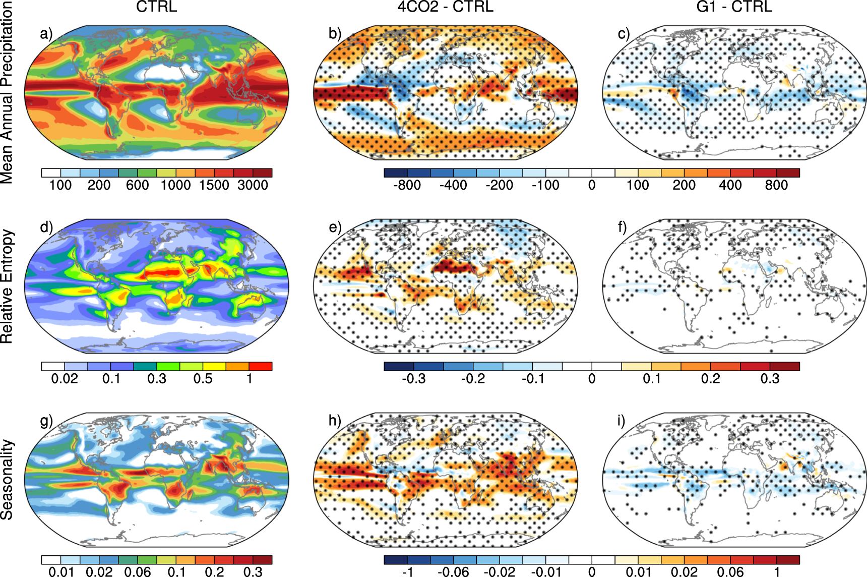
Spatial variations of the mean annual precipitation from the CTRL simulation and their changes in 4xCO₂ and G1 are shown in figures 1(a)–(c). In the CTRL simulation, the highest observed mean annual precipitation is seen over the tropics, where the precipitation amount ranges between 1500–3000 mm/year. Polar regions receive the least annual precipitation along with the hot desert and arid climatic regions of North Africa, South Africa, western India and the Middle East countries, which receive 100–200 mm/year of mean annual precipitation.

**Figure 1.** The spatial pattern of the mean annual accumulated precipitation (mm), relative entropy and seasonality index from the CTRL simulations and changes under 4xCO₂ and G1 with respect to the CTRL are shown in the upper panel (a)–(c), middle panel (d)–(f) and lower panel (g)–(i), respectively. Stippling denotes the two-tailed Student's t-test significant at the level of 95%.
Download figure:
Standard image High-resolution image

In 4xCO₂ simulations, the multi-model mean shows both an increase and decrease in precipitation over different parts of the globe, although the regions with increases significantly outnumber the regions with decreases. The largest increase in precipitation is found over the equatorial Pacific Ocean. A significant increase in precipitation is also seen over the northwest Indian Ocean and many parts of the Arctic and the Antarctic regions. On the other hand, a decrease in precipitation is seen over Mexico and Central America, northern parts of South America and a large fraction of the North Atlantic Ocean. As can be seen from G1 simulations, G1 significantly nullifies the changes seen in 4xCO₂ over most parts of the globe, although there are anomalies of both positive and negative signs over many parts with very small magnitudes. However, some regions, such as the northern part of South America, show a decrease in precipitation under both 4xCO₂ and G1.

3.2. Relative entropy

The spatial variation in relative entropy during the CTRL period and its changes under the 4xCO₂ and G1 scenarios are shown in figures 1(d)–(f). It is observed that, overall, relative entropy is higher over most of the tropical rain belt and few of the subtropical regions and it is more over land than the oceanic region. Within the tropical climatic region, North African and western Indian regions show the highest values of relative entropy (>=0.8). Due to the presence of drier regions, like the Sahara in Africa and the Thar Desert in Rajasthan, relative entropy is higher over these regions. For example, Rajasthan (a state in western India) receives 75%–80% of its annual precipitation during the southwest monsoon season, i.e. during June–September. However, the duration of the southwest monsoon rainfall over Rajasthan is very short due to late arrival and early withdrawal (Sahany et al 2018, Mehfooz et al 2005). Therefore, relative entropy is seen to be high as rainfall is concentrated in a short duration. Few of the mid-latitude regions (eastern US and northwestern Europe) that receive precipitation uniformly throughout the year have low values of $\bar{D}.$ Further, Antarctica (along with the Southern Ocean), Arctic, subarctic or subpolar climatic regions receive low annual precipitation and have low entropy values as precipitation is nearly equally distributed throughout the year.

In the 4xCO₂ scenario, increases in relative entropy are seen over tropical climatic regions, specifically over the landmass of northeastern parts of South America, African sub-continents and South Asia, indicating the lowering of temporal spread in peak precipitation periods. In general, we find an increase in relative entropy in the 4xCO₂ scenario over both land and ocean, but with a slight deviation over mid-latitude regions (eastern US and northwestern Europe), parts of Russia and its adjoining region, where a decrease in relative entropy is projected. However, under G1, relative entropy values are found to be close to those seen in the CTRL simulations, thus, significantly nullifying the impact of 4xCO₂.

3.3. Seasonality index

The spatial variation in the seasonality index $\bar{S}$ during the CTRL period and its changes under the 4xCO₂ and G1 scenarios are shown in figures 1(g)–(i). Variation in the seasonality index may be caused by changes in either relative entropy or the normalized mean annual precipitation, or both. Changes in relative entropy could be due to changes in the monthly distribution of annual precipitation, whereas changes in the normalized annual precipitation could either be due to a change in R or a change in R_max in the two simulations. It is possible that over a given grid point, R as well as $\bar{D}$ are invariant in the two simulations, but due to a change in R_max the seasonality index could turn out to be different. To avoid such misinterpretations, we have used the same R_max (global maximum precipitation of the piControl multi-model mean) for computing the normalized annual mean precipitation in the 4xCO₂ and G1 scenarios.

In the CTRL simulation, $\bar{S}$ values are higher over tropical regions and mid-latitudes, due to the high relative entropy over these regions. The largest values of $\bar{S}$ are generally found over western sub-Saharan and central Africa, northern Australia, parts of east-central South America and South Asia. These regions of high seasonality are embedded within the Asian–Australian, the African and the American monsoon systems (Trenberth et al 2000, Wang and Ding 2008).

Under the 4xCO₂ scenario, the seasonality index shows an increase over most parts of the global monsoon regions, except over Mexico and northwestern South America where it is found to decrease. Over regions showing large increases in seasonality in 4xCO₂ both the mean annual precipitation and entropy show large increases. For example, in parts of southeast Asia, an increase in seasonality values is influenced by an increase in both the mean annual precipitation and relative entropy. Also, an increase in the seasonality index over oceanic regions, such as the eastern Pacific, south equatorial Atlantic and north Indian Ocean, is due to an increase in the mean annual precipitation and relative entropy over these regions. In the G1 simulations, the seasonality index significantly decreases over some parts of the global monsoon regions, including land and ocean, parts of subarctic or subpolar climatic regions (specifically over Canada, Russia and parts of Europe). However, over some regions, such as central east South America, southern Africa and some parts of the western Arabian Sea, the equatorial Pacific and the Atlantic Ocean, geoengineering does not significantly nullify changes in the seasonality index seen in 4xCO₂. Overall, due to solar geoengineering, the offset with respect to the changes seen in the 4xCO₂ scenario are 130%, 96% and 118% for annual precipitation, relative entropy and seasonality index, respectively.

3.4. Centroid of the peak precipitation period

Figures 2(a)–(c) show the spatial variation in the timing of the peak precipitation period for the CTRL and changes under 4xCO₂ and G1 in months. From the CTRL simulation it is found that the centroid of the peak precipitation period is concentrated between July–December over the Northern Hemisphere, while it mainly occurs between January–June in the Southern Hemisphere, with regional variations. Over tropical rain belt regions the precipitation is more concentrated during June–September months (during Northern Hemisphere monsoon seasons). In 4xCO₂, the precipitation peak is projected to shift either forward or backward by 15 days–1 month over many parts of the globe. In particular, over the tropics, the peak is projected to shift forward by 1 month, i.e. from mid-June–mid-July.

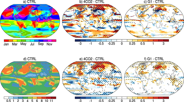
**Figure 2.** The upper panel shows the spatial variation in the timing of the peak precipitation during the peak precipitation period for the CTRL (a), corresponding changes in months under 4xCO₂ (b) and G1 (c) with respect to CTRL. The lower panel shows the spatial pattern of the duration of the peak precipitation period from the CTRL (d), corresponding changes in duration in months under 4xCO₂ (e) and G1 (f) with respect to the CTRL. Stippling denotes the two-tailed Student's t-test significant at the level of 95%.
Download figure:
Standard image High-resolution image

Further, there are slight variations in shifts of the peak from the tropics towards the poles. In comparison to the 4xCO₂ scenario the changes in the peak of the annual precipitation period in G1 are fewer. Over the tropics, the changes in the centroid under G1 are within 15 days backward or forward when compared with the CTRL simulation. Over some of the mid-latitude countries, such as France, Russia, Finland, Denmark, Norway and Sweden (belonging to the subpolar climatic regions), the peaks are shifted by more than 2 months.

3.5. Duration of the peak precipitation period

The spatial variations in the duration of the peak precipitation period from CTRL runs and corresponding changes in duration for 4xCO₂ and G1 are shown in figures 2(d)–(f). From the CTRL simulations, we find that duration of the peak precipitation period is shorter over most parts of the tropical regions. Over the tropics, specifically South Asia, North Africa and Central America regions, the duration of peak precipitation periods varies in the range of 1–5 months. These regions generally get precipitation during their monsoon seasons.

In the case of 4xCO₂, a significant increase in the duration of the peak precipitation period is found over most of the polar and subpolar climatic region, while a significant decrease in the duration of the peak precipitation period is seen over most of the tropical regions. It is projected that the precipitation duration may reduce by 15 days–2 months over some parts of the tropics that include both land and oceans. Specifically, over the Bay of Bengal, Arabian Sea, southern Indian Ocean and North Atlantic region, the duration of the peak precipitation period is projected to decrease by 15 days–1 month, whereas over the eastern Pacific region near to the Peru coast, the duration of the peak precipitation period is projected to increase by 15 days–1 month. In the Northern Hemisphere, particularly over northern Europe and North America, the change in precipitation duration is projected to increase by 1–3 months. G1 simulation largely balances the reduction in the duration of the peak precipitation period. Over polar regions as well as over tropical regions, the change in the peak precipitation period is reduced to 1 month when compared to the 4xCO₂ scenario (which is around 2 months), but over a few regions like North America and Central Europe, the increase in the duration of the peak precipitation period (∼15 days–1 month) in the G1 simulations remains similar to that seen in the 4xCO₂ scenario.

3.6. Regional precipitation variations

Figure 3 shows the monthly variations of area-averaged accumulated precipitation during the CTRL period, 4xCO₂ and G1 simulations. We have selected some sample locations from the global monsoon and tropical storm track regions (based on significant changes in seasonality index, relative entropy and annual precipitation accumulation) to evaluate the annual variations in the precipitation and its peak and duration of the peak precipitation period by comparing the model simulation results from 4xCO₂ and G1 simulations with the CTRL simulations. The global monsoon precipitation regime is defined by the regions where the local summer precipitation exceeds 55% of the annual total (Wang and Ding 2008, Kitoh et al 2013). The monsoon region is distributed globally over all tropical continents, and in the tropical oceans in the western North Pacific, eastern North Pacific and the southern Indian Ocean. Thus, the global monsoon precipitation domain includes all major monsoon regions: Indian summer monsoon (IND, 10N-35N; 67E-97E), East Asian monsoon (EAS, 28N-46N; 115E-125E), western North Pacific monsoon (WNP, 110E-155E; 10N-28N), Australian monsoon (AUS, 110E-150E; 5S-15S), South African monsoon (SAF, 5E-90E;0-30S), South American monsoon (SAM, 30W-80W;5S-30S), North African monsoon (NAF, 25E-30W; 5N-15N) and the North American monsoon (NAM, 50W-125W;0-30N). The results show that noticeable variations in the precipitation intensity and peak precipitation period are observed in many parts of the globe in the 4xCO₂ simulation. For example, over the IND region, the precipitation intensity is decreasing during the peak precipitation period (June–September) in the 4xCO₂ simulation with respect to the CTRL and G1 simulations. The EAS region also shows a decrease in precipitation intensity during the peak precipitation period (May–August) in the 4xCO₂ scenario.

Further, over the SAM and SAF regions, a decrease in precipitation intensity is also found in response to the increased CO₂ concentration. Again, over the NAM region, precipitation intensity decreases in 4xCO₂ simulations during its peak precipitation period (May–October).

Further, we have considered a few of the oceanic regions that include major storm track belts over the Pacific, Atlantic and Bay of Bengal based on the classifications derived by Knapp et al 2010 and the National Oceanic and Atmospheric Administration (NOAA) tropical cyclone climatology report (NOAA NWS report 2011) as follows: North Atlantic Ocean (NAO, 45W-75W;10N-30N), east Pacific Ocean (EPO, 85W-150W; 10N-20N;), west Pacific Ocean (WPO, 15E-120E;10N-30N) and the Bay of Bengal (BoB, 75E-105E;5N-25N). The regions with latitudes and longitudes are specified in figure 3. A noticeable decrease in precipitation intensity is seen: (i) over EPO during the peak precipitation period (July–November), (ii) over WPO during the peak precipitation period (July–November), (iii) over BoB during the peak precipitation period (June–September) in 4xCO₂. The change in precipitation intensity during the peak precipitation period over the global monsoon and storm track regimes due to the response of increased CO₂ is largely suppressed in the G1 simulation.

Also, monthly-accumulated precipitation variations in terms of the standard deviation (error bars in figure 3) are computed to estimate the spread in the individual models with respect to the multi-model mean values over different regions and for different simulations. It is found that the spread in precipitation from their mean is higher in 4xCO₂ simulations in most of the global monsoon regions with a maximum deviation of 70–130 mm/month over IND, AUS, NAF and WNP when compared to the other two simulations. In the case of storm track regions, the spread is more over EPO and BoB in 4xCO₂, with the highest spread of 50–124 mm/month.

Further, we have made inter-model comparisons by analyzing the changes in relative entropy and the seasonality index during CTRL, 4xCO₂ and G1 experiments from the individual models (figures not shown). We found that, in general, across individual models, geoengineering leads to a reduction in the changes projected in a 4xCO₂ world over most of the regions in the variables analyzed, but the degree to which geoengineering is effective in mitigating the changes is not the same in each model. However, the ratio of inter-model standard deviation to the multi-model mean, computed at each grid point in each experiment (CTRL, 4xCO₂ and G1) for each variable shows that the weighted-area-average inter-model spread for any variable is not too far away from the multi-model mean, with the maximum spread (∼40%) seen in seasonality (table 1). Further, we quantify differences across individual models against the multi-model mean on a global scale by computing the root-mean-square difference (RMSD) in CTRL, 4xCO2 and G1 for the mean annual precipitation, relative entropy and seasonality index. The RMSD in the global mean annual precipitation of G1-CTRL for individual models against its multi-model mean, ranges between 62–86 mm year^–1, except for the GISS-E2R, CESM1-CAM5 and HadGE2-ES models ranging between 124–153 mm year^–1 (table 2).

Table 1. Weighted-area-averaged ratios (expressed as %) of the inter-model standard deviation to the multi-model mean of annual precipitation, relative entropy, seasonality index, timing of the peak precipitation and duration of the peak precipitation period in CTRL, 4xCO₂ and G1 experiments.

Experiment/Variable	Annual Precipitation	Entropy	Seasonality	Timing	Duration
CTRL	28.67	35.65	40.34	34.32	14.20
4xCO₂	30.93	39.44	42.55	34.43	15.43
G1	29.92	37.42	42.23	35.30	14.07

Table 2. Global RMSD of annual precipitation, relative entropy, seasonality index, timing of the peak annual precipitation and duration of the peak precipitation period for individual models in CTRL, 4xCO₂ and G1 experiments with respect to their multi-model mean values.

		BNU-ESM	CCSM4	CESM1-CAM5	GISS-E2-R	HadGEM2-ES	IPSL-CM5A-LR	MIROC-ESM	MPI-ESM-LR
Annual Precipitation (mm)	CTRL	237.1	178.6	177.8	363.3	287.2	251.3	307.7	311.6
	4xCO₂	159.5	130.7	211.2	207.5	182.2	195.8	189.5	190.7
	G1	76.9	75.6	153.9	142.3	124.6	62.4	81.3	86.3
Entropy	CTRL	0.11	0.08	0.089	0.141	0.133	0.148	0.117	0.188
	4xCO₂	0.073	0.058	0.094	0.070	0.092	0.086	0.084	0.155
	G1	0.037	0.034	0.063	0.037	0.052	0.042	0.035	0.052
Seasonality	CTRL	0.024	0.023	0.025	0.037	0.049	0.03	0.032	0.034
	4xCO₂	0.018	0.02	0.031	0.024	0.028	0.024	0.025	0.04
	G1	0.008	0.009	0.02	0.012	0.017	0.008	0.008	0.014
Timing (month)	CTRL	1.981	1.575	1.776	1.998	1.955	1.925	1.832	1.79
	4xCO₂	2.578	1.841	2.162	2.226	2.322	2.234	2.139	2.156
	G1	1.483	1.446	1.661	1.639	1.72	1.584	1.293	1.597
Duration (month)	CTRL	0.688	0.419	0.547	0.595	0.586	0.623	0.518	0.544
	4xCO₂	0.614	0.368	0.464	0.485	0.488	0.509	0.509	0.475
	G1	0.213	0.209	0.293	0.245	0.282	0.241	0.255	0.236

Figure 4 shows the normalized precipitation-relative entropy diagram that provides R, D and S values averaged over the regions discussed above. We find the highest values of $\bar{D}$ (0.6–0.8) and S (0.15–0.2) over IND, NAF, WPO and BoB regions and the lowest values of $\bar{S}$ (∼0.02) and $\bar{D}$ (<0.2) over NAO, SAF, SAM and EAS regions in different simulations. It is also observed that the $\bar{D}$ values (∼0.4) and $\bar{S}$ values (0.15) are higher over the AUS region and higher $\bar{S}$ values (0.15) and lower $\bar{D}$ values (∼0.2) are observed over the WNP region with the highest normalized precipitation. Therefore, the changes in seasonality index over a particular region could be due to a change in relative entropy, or a change in normalized precipitation or due to changes in both. Again, a large increase in the CO₂ concentration in the atmosphere has a significant impact on precipitation seasonality that shows increase over most of the regions and we find that solar geoengineering significantly nullifies the changes seen in 4xCO₂.

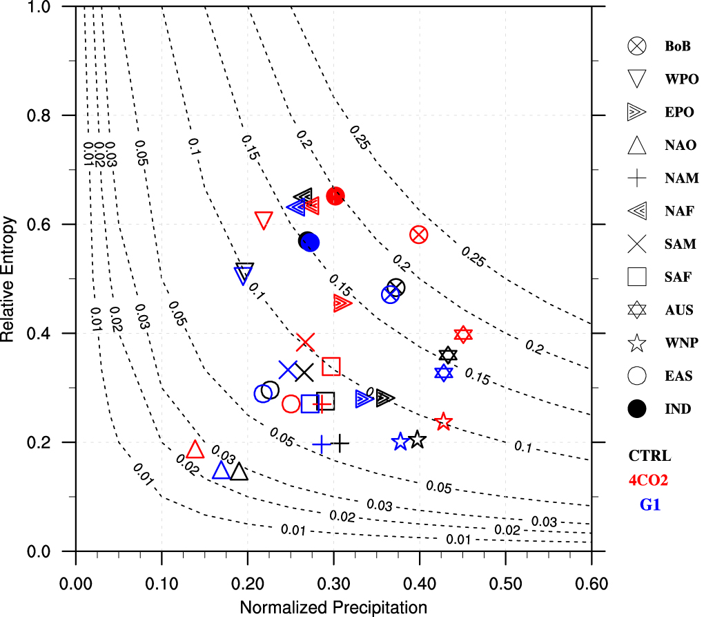
4. Summary and conclusions

In this work we have investigated the impact of quadrupled CO₂ concentration and solar geoengineering on global precipitation seasonality using GeoMIP models. Specifically, we have used dimensionless indicators such as relative entropy and the seasonality index to assess changes in precipitation seasonality. In a 4xCO₂ world, precipitation is projected to increase over many parts of the globe, along with increases in both relative entropy and the seasonality index. A significant increase in precipitation is seen over the equatorial Pacific Ocean, the northern Indian Ocean and many parts of the Arctic and the Antarctic regions. Within the tropics, Indian monsoon and North African monsoon regions show the highest changes in relative entropy and seasonality index along with the west Pacific and Bay of Bengal storm track zones. Also, positive changes in the seasonality index over the eastern Pacific, northern Atlantic, Bay of Bengal and Arabian Sea are projected due to higher values in both the mean annual precipitation and relative entropy. Further, in a 4xCO₂ world the projected change in duration of the peak precipitation period is found to be highest over most of the subarctic climatic region (∼15 days–1 month) including northern Europe and North America. However, over some parts of the tropics, specifically over monsoon regions, it is projected that the precipitation duration may reduce by 15 days–2 months. In 4xCO₂, the precipitation peak is shifted either forward or backward by 15 days–2 months over many parts of the globe, more prominently over the Northern Hemisphere than over the Southern Hemisphere. In particular, the timing of peak precipitation is projected to shift from July–August in some parts and from August–mid-September in some other parts of the tropics. The changes are found in most of the land regions of South Asia, Africa and parts of South America. Solar geoengineering is found to significantly nullify many of the changes projected in a 4xCO₂ world, although there are anomalies of both positive and negative signs over many parts with very small magnitudes.

G1 significantly reduces the precipitation changes seen in 4xCO₂ over most parts of the globe. Relative entropy values are found to be close to those seen in the CTRL simulations, although with small positive and negative deviations over different parts of the globe, thus, significantly nullifying the impact of 4xCO₂. Again, the change in seasonality index decreases over parts of the Arctic, Antarctic and subpolar climatic region. Further, solar geoengineering largely nullifies the reduction in the duration of the peak precipitation period seen over the tropics under 4xCO₂. Over the tropics, the changes in the timing of peak precipitation are within 15 days backward or forward when compared with the CTRL simulation. Over some of the mid-latitude countries; the peaks are shifted by more than 2 months. Thus, we find that there are large projected changes in annual precipitation and its spatio-temporal variability over many parts of the globe in a 4xCO₂ world. However, we find that the implementation of solar radiation management geoengineering significantly nullifies the effects of quadrupled CO₂ on annual precipitation and its spatio-temporal distribution over many parts of the globe. Furthermore, the different models and scenarios used in our study do not always agree in the sign of the change in precipitation, relative entropy and seasonality in response to solar geoengineering. Increased variability in annual precipitation combined with changes in seasonality, due to the increased CO₂ in the atmosphere may likely have a significant impact on agriculture and water resources, with the consequences affecting the economies of many countries in the world. However, solar geoengineering is found to suppress many of these changes seen in the 4xCO₂ scenario. We would, however, like to emphasize that along with investigation of likely changes in annual precipitation and seasonality and its spatio-temporal variability under 4xCO₂ and G1, it is also important to explore likely physical mechanisms behind the noted changes, but this is beyond the scope of our current work and is something which we will be exploring in a follow-up work. We assume that the primary driving mechanism could be: precipitation seasonality is a manifestation of seasonality of temperature (driven by seasonality of solar forcing). Since the spatial gradient in solar forcing between the tropics, mid-latitudes and poles is different in a 4xCO₂ world and G1 (compared to the CTRL), it would lead to different seasonality in temperature, and hence the associated dynamics and precipitation.

Acknowledgments

We acknowledge the World Climate Research Programme's Working Group on Coupled Modelling, which is responsible for CMIP, and we thank the climate modeling groups for producing and making available their model outputs. For CMIP the US Department of Energy's Program for Climate Model Diagnosis and Intercomparison provides coordinating support and led development of software infrastructure in partnership with the Global Organization for Earth System Science Portals. We thank all participants of the GeoMIP and their model development teams, the CLIVAR/WCRP Working Group on Coupled Modeling for endorsing GeoMIP and the scientists managing the Earth System Grid data nodes who have assisted in making GeoMIP outputs available. This research work is partly supported by the DST Centre of Excellence in Climate Modeling (RP02719).

Effects of global warming and solar geoengineering on precipitation seasonality

Article metrics

Submit

Author e-mails

Author affiliations

ORCID iDs

Dates

Peer review information

Abstract

1. Introduction

2. Data and methods