

Export citation and abstract BibTeX RIS

Original content from this work may be used under the terms of the Creative Commons Attribution 3.0 licence. Any further distribution of this work must maintain attribution to the author(s) and the title of the work, journal citation and DOI.
Corrigendum abstract
An error in the estimate of wind plant area led us to underestimate wind power densities by about 40%. The error was our incorrect specification of the geometric projection in the calculation of the area of Voroni polygons in our GIS software. The severity of this error increased with latitude so errors were smaller in Texas than Montana. Our method used area to filter out plants with installed capacity densities <0.1 MWi km−2, a step that generally removes plants with very small numbers of turbines, for which our Voroni method produces overly-large areas. Because the areas changed, the sample set also changed when the error was fixed. Finding the error motivated us to both provide a more detailed description of the method in the supplemental information is available online at stacks.iop.org/ERL/14/079501/mmedia and make data publicly available in an Addendum.
The average wind power density changed to 0.90 We m−2 (from 0.50 We m−2) and the average installed capacity density changed to 2.8 MWi km−2 (from 1.5 MWi km−2). Yet while we are embarrassed to have made an error, these corrections do not affect the overall conclusions of the paper. Specifically: (a) wind plants with the largest areas have the lowest power densities; (b) wind capacity factors are increasing, and that increase is associated with a decrease in installed capacity densities, so power densities are stable or declining; and, (c) the observed average power densities are consistent with prior estimates that use physically-based models of turbine-atmosphere interaction and are inconsistent with many wind resource estimates that implicitly ignore these interactions. Corrections do change figures 3–7 and table 1, as well as text citing or comparing previously incorrect numbers. Paragraphs which required amendments are included below, with corrected numbers and text identifiable as bold-underscored text. We apologize for the inconvenience.
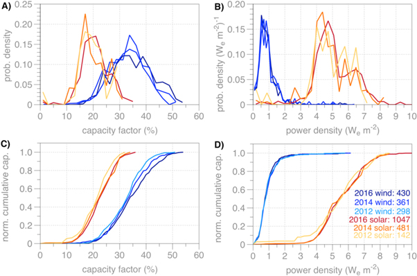
Figure 3. Distributions of capacity factors and power densities. Probability density functions (A), (B) over all wind and solar power plants; and, cumulative distribution functions of the normalized aggregated capacity (C), (D). In each case, annual average data for 2016, 2014, and 2012 is plotted, with the colored key in (D) clarifying wind from solar and the specific year.
Download figure:
Standard image High-resolution image
Figure 4. Age of the power plants compared to their capacity factors, and for wind their power densities. The top bars of (A), (B) show the total capacity of solar or wind power plants for that first year of operation. This first year is also used for binning the capacity factors (A), (B), and power density (B), illustrating how 2016 electricity values were influenced by the power plant's age. Box-whisker plots show the interquartile (IQR) range, white points show the means, red points show the means weighted by the individual power plant's installed capacities for that year, and the red line shows a linear fit through these weighted means. In (B) lower, the black line shows the linear fit from 1984 to 2015, while the red line shows 2006–2015.
Download figure:
Standard image High-resolution image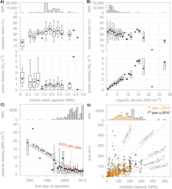
Figure 5. Design characteristics of wind power plants, and their influence on 2016 electricity generation: (A) rated capacity of the wind turbines, (B) capacity density of the wind power plant. The capacity density of wind power plants binned by their first year of operation in (C), with linear fits weighted by the individual power plant's installed capacities for that year for 1984–2015 (black) and 2006–2015 (red). In (A), (B), (C) all box-whisker plots show the interquartile range (IQR), with black dots indicating capacity-weighted mean values. The installed capacity of the wind power plant compared to its area is shown in (D), and uses color to discriminate between wind power plants operational before or after 2010.
Download figure:
Standard image High-resolution image
Figure 6. Spatial distribution of power density (top) and capacity factor (bottom) for 2016. Wind power plants represented as squares and solar power plants as stars.
Download figure:
Standard image High-resolution image
Figure 7. Power densities during 2016, binned by the area of the (A) solar power plant, or (B) wind power plant. Whisker plots show the interquartile range (IQR), with black points showing the capacity-weighted mean of each area bin. Note that the solar areas are about 100-times smaller than the wind power plant areas.
Download figure:
Standard image High-resolution image
Table 1. Solar and wind power values for the various years, with average capacity factor and average power density weighted by the installed capacity.
| Solar power | Wind power | ||||||
|---|---|---|---|---|---|---|---|
| Installed capacity | Capacity factor | Power density | Installed capacity | Capacity factor | Power density | ||
| Year | MWdc | MWac | (%) | (We m−2) | MWi | (%) | (We m−2) |
| 2010 | 78 | 67 | 22.70 | 5.92 | 18 868 | 30.55 | 0.93 |
| 2011 | 218 | 189 | 20.83 | 5.39 | 22 686 | 33.30 | 0.96 |
| 2012 | 833 | 700 | 21.09 | 5.37 | 27 096 | 32.60 | 0.93 |
| 2013 | 2032 | 1692 | 22.87 | 5.72 | 33 529 | 32.47 | 0.92 |
| 2014 | 3518 | 2865 | 23.04 | 5.63 | 34 389 | 33.67 | 0.94 |
| 2015 | 5157 | 4192 | 22.95 | 5.58 | 37 307 | 32.32 | 0.86 |
| 2016 | 8188 | 6612 | 23.52 | 5.70 | 45 400 | 34.94 | 0.90 |
Power density is the rate of energy generation per unit of land surface area occupied by an energy system. The power density of low-carbon energy sources will play an important role in mediating the environmental consequences of energy system decarbonisation as the world transitions away from high power-density fossil fuels. All else equal, lower power densities mean larger land and environmental footprints. The power density of solar and wind power remain surprisingly uncertain: estimates of realizable generation rates per unit area for wind and solar power span 0.3–47 We m−2 and 10–120 We m−2 respectively. We refine this range using US data from 1984 to 2016. We estimate wind power density from primary data, and solar power density from primary plant-level data and prior datasets on capacity density. The mean power density of 430 onshore wind power plants in 2016 was 0.90 We m−2. Wind plants with the largest areas have the lowest power densities. Wind power capacity factors are increasing, but that increase is associated with a decrease in capacity densities, so power densities are stable or declining. If wind power expands away from the best locations and the areas of wind power plants keep increasing, it seems likely that wind's power density will decrease as total wind generation increases. The mean 2016 power density of 1047 solar power plants was 5.7 We m−2. Solar capacity factors and (likely) power densities are increasing with time driven, in part, by improved panel efficiencies. Wind power has a 6-fold lower power density than solar, but wind power installations directly occupy much less of the land within their boundaries. The environmental and social consequences of these divergent land occupancy patterns need further study.
Introduction
Here we estimate the power densities and capacity factors for wind and solar power plants with AC-capacities greater than 1 MW which generated electricity in the US from 1984–2016 installations. For wind we make a direct plant-by-plant bottom-up estimate while for solar our estimates of power density depend on a correlation analysis that provides a single estimate for the solar installed capacity density.
Data sources and methods
Following our Wind and Solar Methods (below), we computed annual averages from monthly generation (MWh/month) when 12 months of data is reported rather than using the data's annual averages (MWh yr−1) which would obscure pre-startup or offline periods. Only about half of all wind and solar power plants were used in our analysis for the year 2016, with this ratio varying by technology and year. These solar and wind power plants were excluded because: (a) Power Plants could not be linked to Electricity Generation based on Plant Code, or (b) Capacity factors calculated from the Power Plants and Electricity Generation exceeded 100%, or (c) Electricity Generation was zero for any month in a given year, or finally (d) AC-capacities between Power Plants and Detailed Data differed by more than ±10%.
These exclusions and filtering result in discrepancies between our dataset and those of the EIA (2018d). For 2016, the cumulative capacity of the wind power plants include in our data was 56% the EIA's estimate for total wind capacity while for solar capacity that figure was 44% (EIA 2018d). Our base Power Plants data collated power plants through early 2018, but does not specify when the power plant came online, preventing capacity for 2016 from being quantified. Detailed Data provides nameplate capacity and month-year per power plant, but for 2016, total capacities are 109% and 150% the capacity for wind and solar respectively compared to (EIA 2018d). To verify that no region was systematically excluded, we spatially compared the raw EIA Power Plant locations (EIA 2018a) to those making it through our methodology, and found no obvious spatial gaps.
Wind methods
A detailed step-by-step methodology is described in the supplemental information, but broadly our approach for quantifying the area of US wind power plants begins with the location of the 57 636 wind turbines in the USWTDB (Hoen et al 2018). The USWTDB was reprojected to Contiguous USA Albers Equal Area (EPSG:102003) to enable precise small-area calculations across latitudes. Voroni polygons were calculated for each wind turbine using QGIS (2018). Using spatial linking, the Voroni polygons were linked to the Power Plants (EIA 2018a) and then filtered for an equivalent AC-installed capacity within ±10%. The Plant Code in the Power Plants data was then used as the unique identifier for linking to Electricity Generation (EIA 2018a, 2018b) and Detailed Data (EIA 2018c). Capacity factors (MWe/MWi) of wind power plants are calculated from Electricity Generation and Power Plants (EIA 2018a, 2018c). Spatial and temporal curtailment by the grid operator was not included in this analysis, but will influence the results slightly (e.g. ERCOT region of Texas in 2009).
There is no well-established method to compute the area of each wind power plant. To do so, we compute a Voroni polygon (after Гео́ргий Вороно́й) using QGIS (2018) for each wind turbine in the USWTDB which delineates the ground area that is closest to each individual turbine location compared to every other turbine. The Voroni polygon areas for wind turbines on the edge of wind power plants are very large, but the interior Voroni polygons are a useful quantification of the ground surface area per turbine. We compute the median Voroni polygon area for each wind farm in the Contiguous US and then estimate the area of the wind farm by multiplying this median Voroni polygon area by the number of wind turbines listed in the USWTDB (Hoen et al 2018).
These steps yield the wind power plant area (km2), power density (We m−2), installed capacity density (MWi km−2), and capacity factor for 430 wind power plants operating in 2016 (45.4 GWi).
Solar methods
Our solar dataset begins with Power Plants (EIA 2018a). Using the unique Plant Code, we linked this file to Electricity Generation (EIA 2018b), resulting in 1 311 solar PV power plants. To reduce errors, we compare the installed capacity (MWac) values with the same Plant Code between Power Plants and Detailed Data (EIA 2018a), excluding the solar power plants that differ by ±10%, leaving 1047 solar power plants for our 2016 analysis (6.6 GWac, 8.1 GWdc).
Results
Distributions of power densities and capacity factors are shown in figure 3. Considering capacity-weighted data for all power plants operational during 2016, the summary results are as follows. The mean and 90-percentile power densities for wind are 0.90 and 1.48 We m−2, while the corresponding values for solar are 5.7 and 7.5 We m−2. Note that systematic uncertainty in the distribution of power densities are significantly larger for solar than for wind because the solar power results are derived from a fixed estimate of capacity density, whereas the wind results are computed directly. Our mean and 90-percentile capacity factors are 34.9% and 46.0% for wind, while the corresponding values for solar are 23.5% and 30.0%. Note that the capacity factors from EIA for 2016 are 34.5% for wind and 25.1% for solar (EIA 2018d), and we expect that the discrepancy arises from the data sampling issues discussed above. Solar and wind power installed capacities, power densities, and capacity factors from 2010 to 2016 are shown in table 1.
Capacity factors for wind power have increased by 0.9% per year over the years 1984–2015 (figure 4(B)). The increase in wind's capacity factor is particularly evident this decade. Wind farms operating since 2010 have a mean capacity factor of 37.3% for 2010–2016, whereas the capacity factor from 1984 to 2009 is 31.6%.
There is no significant trend in the power density of wind power plants. This result is surprising given the increase in capacity factor. What underlies it? Wind power plants have three defining characteristics: the rated capacity of individual turbines, the installed capacity density of the wind farm, and the area of the wind farm. The capacity factor and power density of the wind power plants show no relationship to the rated capacity of the individual wind turbines (figure 5(A)), whereas capacity factor and power density do vary with capacity density (figure 5(B)). Note that the highest power densities are achieved with the highest capacity densities, but the highest capacity factors are achieved with the lowest capacity densities. Based on their first year of operation, the capacity density of wind power plants has decreased by 3.3% per year since 1984, or 3.2% per year over the last 10 years (figure 5 (C)). The capacity density peaked at about 5 MWi km−2 for turbines installed between 2002 and 2005, and has since decreased to about 2.0 MWi km−2. Overall, the average installed capacity density of all wind farms was 2.7 MWi km−2 (figure 5(D)). In summary, we find that while improved wind turbine design and siting have increased capacity factors (and greatly reduced costs) they have not altered power densities.
Finally, we examined the relationship between power plant area and power density. For solar, there is no clear relationship between area and power density (figure 7(A)), whereas for wind, there is a strong relationship (figure 7(B)). While many wind power plants with areas less than 20 km2 generate more than 1.0 We m−2, power density decreases with increasing power plant size. This result was previously observed for 0–20 km2 wind power plants by (MacKay 2013). We verify this early result, and extend it by showing that wind's power density reaches an asymptote of about 0.50 We m−2 when the wind plant area exceeds about 150 km2. Note that we found power densities of about 0.1 We m−2 for the largest wind-farms in our study, which had areas of 250–450 km2. While these plants passed all the quality-checks of the Wind Method, we feel they are not representative. While these plants have comparable capacity factors (24%–47%), they have very low capacity densities (0.11–0.23 MWi km−2). These plants are, in general, isolated from neighboring plants and/or have turbines placed along ridgelines, which is problematic for quantifying a representative median Voroni polygon area. We therefore judge that the power densities of about 0.50 We m−2 in figure 7 (B), which we find for plants of 100–200 km2, as most illustrative to what would likely be achieved by replicating existing wind plants in adjacent regions with similar wind resources.
Discussion
Solar's mean power density in 2016 was 5.7 We m−2. Our approach for estimating the area of solar farms is not fully bottom-up so this estimate is subject to systematic error. It is possible, for example, that capacity densities have changed significantly given that the data used in our analysis is about 5 years old. That said, the assumption by (Jacobson et al 2018) that urban rooftops can be retrofitted with a capacity density 4.5 times higher than the commercial-scale solar plants measured by (Ong et al 2013) seems highly unlikely, as does the resulting 24–27 We m−2 power density (Jacobson et al 2018). It is also possible that capacity densities vary strongly with larger size installations (see figure 2(A)). However, given that our analysis finds only a very weak relationship between module efficiency or installation size and capacity density, we expect the errors are small, likely less than 20%.
Wind's mean power density in 2016 was 0.90 We m−2. This observed mean is consistent with estimates based on atmospheric theory and modeling (Gustavson 1979, Keith et al 2004, Wang and Prinn 2010, Miller et al 2011, Gans et al 2012, Jacobson and Archer 2012, Marvel et al 2012, Adams and Keith 2013, Miller et al 2015, Miller and Kleidon 2016) which predicted that large-scale wind power densities would be under 1.0 We m−2 and also that power densities will decrease with increasing size of the wind farm installation. This observed mean power density is much smaller than many common estimates (Archer and Jacobson 2005, Lu et al 2009, Sta. Maria and Jacobson 2009, Jacobson and Delucchi 2011, Lopez et al 2012, US DOE 2014, World Bank Fund 2018). Examples include 227 W m−2 over the windiest 10% of global land (World Bank Fund 2018), 3.3 We m−2 over the entire Earth's surface (Jacobson and Delucchi 2011), 1.7 We m−2 over about 1/3 of the Continental US (Lopez et al 2012), or 1.4 We m−2 over about 2% of the US with excellent wind resources (US DOE 2014). These are also by no means the highest estimates in the literature. For example, (World Bank Fund 2018) quantify a wind power density of 808 W m−2 over the windiest 10% of US land, and (Kammen and Sunter 2016) estimated an upper bound of 35 We m−2 for wind power at urban-scales based on a study observing numerous vertical axis turbines which generated up to 47 We m−2 over an area of about 50 m2 (Dabiri 2011).
There are two main reasons for these discrepancies in wind power density. First, many estimates did not account the interactions between wind turbine arrays and the atmospheric boundary layer. The limit to large-scale wind power density is the downward flux of kinetic energy from the free troposphere, a global value that is about 1 W m−2 (Lorenz 1955, Peixoto and Oort 1992, Kim and Kim 2013). The effect of this atmospheric limit is illustrated by the relationship between wind power plant's area and power density. Second, many studies assume installed capacity densities which are too high. While we observed an average capacity density of 2.7 MWi km−2 with about 2.0 MWi km−2 common to 2013–2015 installations, (Rinne et al 2018) assume 5.5–9.4 MWi km−2, (Jacobson et al 2018) assume 7.2 MWi km−2, (Lopez et al 2012) assumed 5.0 MWi km−2, the US-DOE Wind Vision: A New Era for Wind Power in the United States (US DOE 2014) assumed 3.0 MWi km−2. By assuming 2–5 times the observed capacity density but ignoring the atmospheric limits, these estimates resulted in power densities that are 2–5 times higher than observations.
Given that larger wind power plants have smaller power densities and given that a major increase in total wind power generation will presumably require expanding wind power plants into less-than-ideal locations, it seems likely that wind power density will decrease with time. It therefore seems—contrary to many prior estimates—unlikely that the power densities of greater than 1 We m−2 will be realized over substantial areas, and likely that average power densities of about 0.5 We m−2 will become increasingly common.
As an example of the implications of these results, consider Germany and its ambitious energy transformation policy (Energiewende). Germany's primary energy consumption rate is 1.28 W m−2 (BP 2018). If the average US wind power density of 0.90 We m−2 was applicable to Germany, then devoting all German land to wind power would meet about 70% of Germany's total primary energy consumption, while if German wind power performs like the best 10% of US wind (1.48 We m−2), then generation would be 115% of Germany's consumption. Finally, if Germany's goal was to generate the most wind power without economic constraints, very high capacity densities (e.g. 10 MWi km−2) could be deployed, reducing capacity factors but possibly raising the power density to 2.0 We m−2 and meeting 135% of consumption. Whereas for solar at 5.7 We m−2, 22% of Germany's land area would need to be devoted to commercial-scale solar to meet total primary energy consumption.
Power densities clearly carry implications for land use. Meeting present-day US electricity consumption, for example, would require 12% of the Continental US land area for wind at 0.5 We m−2, or 1% for solar at 5.7 We m−2. US electricity consumption is just 1/6 total primary energy consumption (BP 2018), so meeting total consumption would therefore require 72% and 6% respectively for US wind and solar. Of course, like the Germany example, no single energy source is likely to ever supply all electric power. These comparisons nevertheless provide a benchmark for understanding the implications of power densities for land use, while recognizing that solar and wind power also occupy the area within the power plant boundary differently. These observation-based results should be considered in light of the fact that (a) decarbonizing the energy system will require considerably more primary power than current electricity demand, (b) demand may continue to grow, and finally, (c) that many areas of the world have higher energy demand per unit area than does the Continental US.