

Abstract
Do food imports increase the variability of domestic food prices? The answer to this question depends on whether foreign production is more volatile than domestic production. If imports are likely to destabilize domestic prices, storing crops for future consumption may prove an appealing strategy to cope with the adverse supply effects of a more unstable climate. Unfortunately, public storage has proven to be unsustainable due to the high costs of carrying crop inventories over time and the inability of policy planners to correctly forecast changes in domestic supply. Therefore, understanding the roles of imports and stocks on domestic food price instability is important as domestic shortfalls in food production are likely to become more frequent as the world's climate becomes warmer. Using maize prices observed in 76 maize markets of 27 maize net importers across Africa, Asia and Latin America during 2000–2015, we find that, on average, a 1% increase in the ratio of imports to total consumption is correlated with a 0.29% reduction of the intra-annual coefficient of variation of maize prices; likewise a 1% increase in the amount of maize available in stocks at the beginning of the season is correlated with a 0.22% reduction in the said coefficient. We also find that climate-induced supply shocks toward mid-century may increase maize price variability in the focus countries by around 10%; these increases could be offset with similar increases in the ratio of imports to total consumption or in the stock-to-use ratio at the beginning of the crop marketing year. The fact that both imports and stocks help to stabilize domestic prices suggests that their uses should hinge on a careful cost-benefit analysis, including the risk of facing world production more variable than domestic production and the costs of carrying maize inventories over time.

Original content from this work may be used under the terms of the Creative Commons Attribution 3.0 licence. Any further distribution of this work must maintain attribution to the author(s) and the title of the work, journal citation and DOI.
1. Introduction
International trade in agricultural products has grown rapidly since the early 1980s, with many developing countries becoming net importers of cereals and other staples (Valdes and Foster 2012, Rakotoarisoa et al 2011, Porkka et al 2013, OECD/FAO 2018). By spreading the sources of supply of a given market over a larger group of suppliers, trade can serve as a risk sharing mechanism (Bigman 1986). Therefore, imports could help to reduce domestic price instability by supplementing domestic markets at times of adverse domestic supply shocks. However, imports also increase the vulnerability of domestic markets to supply shocks originated overseas (Puma et al 2015, Ceballos et al 2016, d'Amour et al 2016, Gephart et al 2016, Marchand et al 2016, Seekell et al 2017), a possibility exacerbated by the fact that agricultural exports of main staples are concentrated in a handful of countries like the US (Brooks et al 2013, d'Amour et al 2016, Challinor et al 2017).
Regardless of export concentration, whether imports reduce or increase domestic price instability depends on whether international markets are more volatile than domestic markets (Díaz-Bonilla 2015). Deaton and Laroque (1992)'s seminal characterization of commodity prices indicates 'rare but violent explosions in prices, coupled with a high degree of price autocorrelation in more normal times.' In world agricultural markets, this behavior takes the form of long periods of relatively stable prices interrupted by sudden price spikes, such as those in the second half of the 2000s (Abbott 2012). In contrast to world markets—where supplies of many countries are pooled—domestic markets are subject to the localized vagaries of weather every single season; therefore, prices determined in isolation from world markets and absent any other price stabilization policy (e.g, floor prices in India (Villoria and Mghenyi 2016)) are more likely to show greater levels of instability than those in world markets. Empirical evidence from Brown and Kshirsagar (2015), for instance, shows that food price variations in the developing world were mainly attributable to local weather-induced crop yield shocks, rather than to international price shocks.
An alternative way to stabilize domestic markets is to use public buffer stocks, whereby, a government agency intervenes by buying domestic excess supplies in years of good crops in order to increase domestic prices; likewise, the release of stocks in years of bad crops helps to mitigate price spikes (Williams and Wright 1991). Most countries use a mix of buffer stocks and variable trade policies to stabilize markets (Williams and Wright 1991, Demeke et al 2009). Stocks, however, are costly and inefficient (Díaz-Bonilla 2017), often leading to spoilage and high costs of keeping inventories. Advocates of international trade point out to these costs as a main argument to use international markets as a way to stabilize prices (Bigman and Reutlinger 1979).
Previous studies have used model simulations to examine the impacts of trade and buffer stocks on the stability of domestic food prices (Bigman and Reutlinger 1979, Williams and Wright 1991, Miranda and Glauber 1995, Makki et al 2001). Some used case studies in Bangladesh, Mexico, Malawi and Zambia (Dorosh 2001, World Bank 2005) and cross-sectional comparisons (Chapoto and Jayne 2009, Minot 2014) with a focus on trade. Yet, none of them has estimated the functional relationship of imports on domestic food price stability. To fill this gap, the objective of this letter is to estimate the effects of imports and buffer stocks on the intra-annual coefficient of variation (CV) of real monthly prices of maize in a group of net food-importing countries in Africa, Asia, and Latin America. We focus on maize, because it is a major staple that is widely produced, consumed and traded around the world (Ranum et al 2014), and its domestic prices are highly variable in many developing countries (Minot 2014).
Crop yields will likely become more variable under climate change (Challinor et al 2014, IPCC 2014, Villoria and Chen 2018), with some authors documenting the potential for more variable domestic prices (Haile et al 2017). In light of this, we explore the roles of international trade and buffer stock in mitigating the potential greater price variability associated with a more unstable climate.
2. Methods and data
We proceed in two steps. First, we use regression analysis to estimate the effects of domestic yield shocks, imports, and buffer stocks on the intra-annual CV of real monthly prices of maize in 27 countries, most of them low- or middle-income. Second, we use the parameter estimates from the regression to examine future scenarios of maize price variability under alternative projections of maize yields toward mid-century. We also explore the potential of increasing maize imports and maize buffer stocks to counteract the price effects of more variable yields stemming from a more variable climate.
2.1. Estimating the effects of domestic supply shocks, import dependence, and buffer stocks on price variability
The data used for estimation, described below, have a panel structure with 76 sub-national markets (denoted by k) in 27 countries (denoted by i) observed during the 2000–2015 marketing years, denoted by t. With these data, we estimate the following regression:

where CVik,t is intra-annual CV of real monthly prices of maize in kth market of country i at year t.
Our main interests are the parameter estimates of α1, α2, and α3. The data used to estimate these parameters are: the national annual ratios of net imports (i.e. imports minus exports) to domestic consumption, Ii,t; the annual absolute yield deviations from historical trends1 in each country i, Yi,t, which captures the effects of both positive and negative domestic supply shocks on domestic maize price instability; and the country-level stock-to-use ratio at the beginning of the marketing year t, Mi,t. The and are vectors of control variables and their corresponding parameter estimates that have direct effects on domestic price stability, namely, exchange rate variability (Cho et al 2002), food aid (Barrett et al 1999, Lentz et al 2005) and social conflict (Bellemare 2015). In addition, as discussed below, the robustness of our results is explored by controlling for other variables that could be correlated with both price variability and import ratios, including physical trading distance, degree of import diversification, and per capita income (Luan et al 2013, Jeon and Ahn 2017).


We also exploit the panel nature of our data to control for unobservables. Specifically, the terms μi and δk denote country and market fixed effects, which control for time-invariant, unobserved country and market heterogeneity. The term ϕt is a year fixed effect that controls for the unobserved shocks affecting all the markets within a given marketing year. These account, for instance, for the excessive volatility that characterized the period 2005–2012 (Abbott 2012). The term  ik,t denotes residuals, assumed to be normally and independently distributed, as well as uncorrelated with the independent variables. Equation (1) is estimated using a fixed effects, panel data regression estimator—also known as Least Squares Dummy Variable—as described in Greene (2011, p.287).
Table 1 describes data sources and definitions of the regression variables in equation (1). Table 2 reports their descriptive statistics. The dependent variable is annual CV of real monthly prices of maize (in 1982–1984 US dollars) obtained from the FAO GIEWS database (FAO 2017). We focus on 76 retail or wholesale markets in 27 countries in the FAO GIEWS database that are net importers of maize. These countries are in Asia, Africa, and Latin America. The data are available from 2000–2015 (see appendix tables S1–S2, figure S2). Cumulative maize imports during 2011–2015 of these countries accounted for nearly one third of maize global imports. Figure 1 shows the 2000–2015 averages of intra-annual CV of real monthly maize prices, net import ratios, and stock-to-use ratios at the beginning of the marketing year for all the focus countries. At a glance, this map suggests that, generally speaking, countries with relatively low imports (e.g. those in Africa and Asia) tend to display more variable prices.

Figure 1. Maize price variability, imports and buffer stocks across focus countries. Data source: PS&D online database (USDA 2017).
Download figure:
Standard image High-resolution imageTable 1. Definitions of regression variables and data sources.
| Variable name | Definition | Data source |
|---|---|---|
| Domestic price variability (dependent variable) | Intra-annual coefficient of variation of real monthly prices (in 1982–1984 US dollars) within a country-specific marketing year. | Prices: FAO Global Information and Early Warning System (FAO 2017); Marketing year: PS&D online database (USDA 2017). |
| Net import ratio | Net imports (imports- exports) divided by consumption. | PS&D online database (USDA 2017). |
| Beginning stock-to-use ratio | Stocks available at the beginning of marketing year divided by consumption. | PS&D online database (USDA 2017). |
| Absolute yield deviations | Absolute yield deviations from historic trends divided by trend values. Trends are fitted by HP filter (Hodrick and Prescott 1997) with smoothing parameter of 100. | FAOSTAT (FAO 2018). |
| Variability of real exchange rate | Intra-annual coefficient of variation of real exchange rate within a country-specific marketing year. Calculations of real exchange rates follow Villoria and Hertel (2011, p. 921). | Exchange rates: exchange rate archives of International Monetary Fund and OANDA website.a Consumer price index: FAOSTAT (FAO 2018). |
| Food aid ratio | Food aid divided by consumption. | Food Aid Information System of the World Food Programme (WFP 2018). |
| Social conflict | A dummy variable that is 1 if the use of armed force results in at least 25 battle deaths in a year and 0 otherwise. | Social Conflict in Africa Database (Salehyan et al 2012). |
| Import distance | Import share weighted distance between the importing country and its trading partners. | Trade data: Global Agricultural Trade System (USDA 2018); Distance data: CEPII (Mayer and Zignago 2011). |
| Herfindahl index of import shares | Sum of squared bilateral import shares. | Global Agricultural Trade System (USDA 2018). |
| Per capita GDP | GDP divided by the population. | World Bank open data system.b |
aThe website link is https://oanda.com/currency/average. bThe website link is https://data.worldbank.org/.
Table 2. Summary statistics of regression variables. Notes: there are much fewer observations for food aid ratio because data on food aids during 2013–2015 are not included in the source database. The units for import distance and per capita GDP are thousand kilometers and thousand U.S. dollars, respectively. Other variables do not have units.
| Number of obs. | Mean | Median | Standard deviation | Min. | Max. | |
|---|---|---|---|---|---|---|
| Domestic price variability | 851 | 0.13 | 0.11 | 0.08 | 0 | 0.52 |
| Net import ratio | 851 | 0.25 | 0.11 | 0.3 | −0.19 | 1.06 |
| Beginning stock-to-use ratio | 851 | 0.09 | 0.09 | 0.06 | 0 | 0.5 |
| Absolute yield deviation | 851 | 0.09 | 0.05 | 0.1 | 0 | 0.56 |
| (HP filter) | ||||||
| Absolute yield deviation | 851 | 0.11 | 0.07 | 0.11 | 0 | 0.61 |
| (Quadratic) | ||||||
| Social conflict | 851 | 0.17 | 0 | 0.37 | 0 | 1 |
| Variability of real | 851 | 0.03 | 0.02 | 0.02 | 0 | 0.11 |
| exchange rate | ||||||
| Food aid ratio | 631 | 0.01 | 0 | 0.03 | 0 | 0.34 |
| Import distance | 808 | 0.41 | 0.35 | 0.24 | 0.02 | 1.56 |
| Herfindahl index of | 808 | 0.72 | 0.75 | 0.25 | 0.19 | 1 |
| import share | ||||||
| Per capita GDP | 808 | 3.72 | 1.93 | 4.42 | 0.22 | 32.99 |
A different perspective on these data is in figure 2, which plots the 2000–2015 average intra-annual CV of real monthly maize prices against import ratios in all the focus countries2 . This figure shows that African and Asian countries have low import ratios (less than 0.1) and highly variable maize prices (Morocco is an exception). China, on the other hand, has a low import ratio and also the lowest levels of price variability among the focus countries, probably reflecting the effects of price stabilization policies (Pieters and Swinnen 2016, Chen et al 2018). Compared with the countries in Asia and Africa, the countries in Americas have higher import ratios and lower intra-annual CVs of their maize real prices.

Figure 2. Relationship between maize price variability and maize import ratio across focus countries.
Download figure:
Standard image High-resolution image2.2. Predicting future price variability
To predict the variability of future maize prices in each market, we proceed as follows. First, we obtain time series of maize yields (in tonnes per hectare) for the period 2006–2050 from two alternative sources: the yield-climate response function estimated by Moore et al (2017) and two of the global crop models from the GGCMI-AgMIP archive (Elliott et al 2014, Rosenzweig et al 2014)3 .
Moore et al (2017)'s function is a meta-analysis regression of a large database on crop yield changes compiled by Challinor et al (2014). This function relates changes in temperature, precipitation, CO2 concentration, and on-farm management to changes in crop yields of several crops. The parameter estimates of this response function are global (see appendix section S1); therefore, variability in yield responses at any resolution other than global (e.g. gridcell or country) comes solely from regional variability in climate and the other explanatory variables. Moore et al (2017) used this function, jointly with data of future climate, to estimate high-resolution yields for the entire world. In an analogous manner, we use the their parameter estimates to predict country-level maize yields for each year in 2006–2050.
For this, we use data on temperature and precipitation from the ensemble of five global circulation models included in the GGCMI-AgMIP archive (Hempel et al 2013, Warszawski et al 2014), aggregated to the growing season of each focus country by Villoria et al (2018). Moreover, we obtain predictions with and without the effects of CO2 fertilization, using the data on temperature to infer CO2 concentrations as indicated in Moore et al (2017) (see appendix section S1 for details)4 . We also obtain projected yields with and without CO2 from the GGCMI-AgMIP archive (Elliott et al 2014, Rosenzweig et al 2014), aggregated both to the country-level and to the growing season of each country using the GGCMI-AgMIP interface by Villoria et al (2016). To be consistent with the treatment of the maize yield shocks used to estimate equation (1), we calculate absolute projected maize yield deviations from their trends (see footnote 1). We denote these absolute deviations as , for t in 2006–2050.

Second, we combine these future yield deviations with the parameter estimates of equation (1); this procedure yields the corresponding predicted intra-annual CV of real monthly prices of maize in each focus market for each year in 2006–2050. In the analysis below, we will contrast our predicted scenarios of price variability against historical price variability. The most obvious measure of historical price variability in our study are the observed intra-annual CV of real monthly maize prices used to estimate equation (1). However, historical maize yield variability explains only some of the observed variance of past real maize prices while our predictions are solely driven by yield fluctuations. In order to circumvent this difficulty, we use absolute deviations from trend (see footnote 1) of observed maize yields during 1961–2014, denoted by , to predict the historical intra-annual CV of real monthly prices of maize in each focus market. These are directly comparable with the future predictions.

Formally, we get the historical () and future () predictions using:


and
where hat indicates that these are the parameters estimated in equation (1), or their predicted values. The rest of the variables are set to their means over 2000–2015. For example, is the average import ratio of country i during 2000–2015. In addition, and are intercept estimates specific to each country i and market k, and is the estimated value of the fixed effect for year 2015. In other words, our predictions of both historical and projected CV of maize prices assume that the rest of the variables remain constant, and therefore, they exclusively capture the effect of historical and projected yield variability on price variability.


3. Results
3.1. Import dependency reduces domestic price variability
To aid with interpretation, figure 3 reports our regression results as elasticities evaluated at their sample means, with 95% confidence intervals generated by the Delta method (appendix section S3). The underlying parameter estimates are reported under column 'Model 4' in appendix table S3. These elasticities measure percentage changes in the intra-annual CV of monthly real maize prices given one percentage change in a given independent variable.

Figure 3. Elasticities of the intra-annual CV of real monthly maize prices to changes in the determinants of price volatility included in equation (1). Notes: the error bars represent 95% confidence intervals. The underlying parameter estimates with yields detrended by HP filter are reported in column 'Model 4' in appendix table S3. The underlying parameter estimates with yields detrended by quadratic regressions are reported in column 'Quadratic' in appendix table S6. An elasticity is defined as the percentage changes in the intra-annual CV of real monthly maize prices, given one percentage change in a given independent variable.
Download figure:
Standard image High-resolution imageStarting with the effects of yield shocks, our estimates suggest that a 1% increase in the absolute deviation of annual maize yields from their historical trend, is associated with a statistically significant increase of 0.09% in the intra-annual CV of real monthly maize prices. Also, a 1% increase in maize stocks relative to maize consumption at the beginning of the marketing year, is associated with a reduction of the intra-annual CV of real monthly maize prices of 0.22%. Regarding imports, an increase of 1% in the ratio of maize imports to total consumption is associated with a decrease in the intra-annual CV of real monthly maize prices of 0.29%. In short, our findings are aligned with the expectation that domestic maize supply shocks are a source of maize price fluctuations. They also confirm that larger import ratios and stock inventories at the beginning of the year are associated with lower price instability in the focus countries.
In appendix table S4, we show that these findings are robust to estimations using different time periods, to the omission of years with either high or low international prices, to alternative calculations of domestic supply shocks and to additional controls such as physical import distances, import diversification and per capita income. In appendix table S5, we show that these results are robust to estimation focused on different geographic regions, to the inclusion of countries with high or low import ratios, and to the inclusion of countries with large or short distances to their trading partners.
3.2. Future maize prices are expected to become more unstable
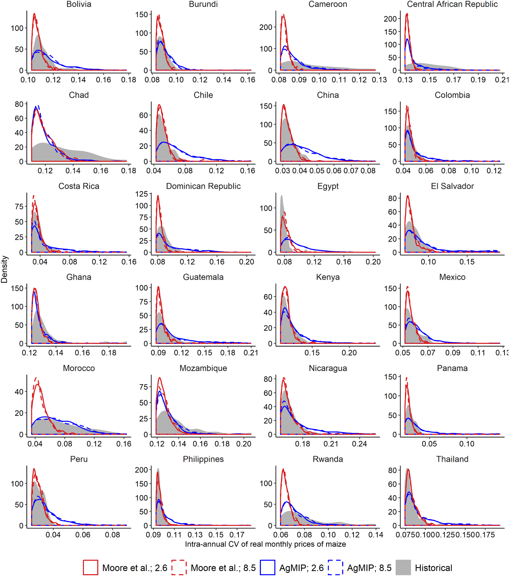
Figure 4 displays, for each focus country5 , the density distributions of market-average intra-annual CV of real monthly prices of maize in the historical period (1961–2014), from equation (2), and in the projected period until mid-century (2006–2050), from equation (3). The price projections in this figure were obtained using projected yields assuming no effects of increased CO2 fertilization under RCP 2.6 and 8.5 6 . The most consequential finding in this figure is that the two sources of projected maize yields produce conflicting views of future scenarios of price instability. In particular, the GGCMI-AgMIP crop models predict that, in 17 out of 24 focus countries, maize prices will become more variable over the coming decades, which is evidenced by the more right-skewed density curves over the projection period 2006–2050. In contrast, the yield response function from Moore et al (2017) predicts that maize prices will become less variable in almost every focus country, relative to the historical densities (appendix figure S8 shows a case for Kenya).


Figure 4. Distributions of projected intra-annual CV of real monthly prices of maize during 2006–2050 without CO2 fertilization and in historical times (1961–2014). Notes: results for Ecuador, Honduras and Israel are not shown due to lack of observed crop calendar data to aggregate the projections of temperature and precipitation (Sacks et al 2010). The results with CO2 fertilization are shown in appendix figure S4.
Download figure:
Standard image High-resolution imageThe conflicting views on prices are rooted in very different projections on future yield variability from the two modeling frameworks. Specifically, visual inspection of figure 5 reveals that the GGCMI-AgMIP crop models predict increases in maize yield variability in most countries. In contrast, the meta-analysis yield response function from Moore et al (2017) predicts density functions that are less spread than the density of historical yields.

Figure 5. Distributions of detrended maize yields during 2006–2050 without CO2 fertilization and in historical times (1961–2014). Notes: maize yields are detrended by the HP filter (Hodrick and Prescott 1997) with a smoothing parameter of 100. Historical yields are from FAOSTAT (FAO 2018), and future yields are projected by GGCMI-AgMIP crop models (Elliott et al 2014, Rosenzweig et al 2014) and Moore et al (2017)'s yield-climate response function in combination with five global climate model ensembles used by the Inter-Sectoral Impact Model Intercomparison Project (Hempel et al 2013, Warszawski et al 2014). Results for Ecuador, Honduras and Israel are not shown due to lack of observed crop calendar data to aggregate the projections of temperature and precipitation (Sacks et al 2010). The results with CO2 fertilization are shown in appendix figure S9.
Download figure:
Standard image High-resolution imageWe surmise that this reduction in maize yield variability owes to the fact that nearly 70% of the data points in the underlying database used by Moore et al (2017), are for the US and China (supplementary table 1 in Challinor et al 2014). Countries in tropical regions, which are more sensitive to warming (Porter et al 2014, Challinor et al 2014), are much less represented. As noted by Moore et al (2017, p.3) 'our meta-analysis results are more optimistic in tropical areas' than the GGCMI-AgMIP crop models—in fact, their projected yield losses are 5 to 50% lower than those projected by the GGCMI-AgMIP crop models within the tropical regions (see supplementary figure 6 in Moore et al (2017)). Such a reduction in yield variability is at odds with the expectation that future yields will become more variable because of more variable temperature and precipitation7 (Chen et al 2004, McCarl et al 2008, Porter et al 2014, Müller and Robertson 2014, Haile et al 2017). In light of this discussion, we will use the prices projected using GGCMI-AgMIP yields in the discussion that follows. We notice, however, that these data have some well known caveats. For instance, the GGCMI-AgMIP crop models use simplistic assumptions about the distribution of soils, sowing dates, varieties and fertilizers, which can affect the temporal dynamics in the yield projections (Müller et al 2017). Nor do these models capture weather-related pest or disease outbreaks that could constitute short-term yield shocks (Rosenzweig et al 2014, Müller et al 2017).
4. Discussion and limitations
To discuss the implications of our results, we investigate by how much could countries increase either their maize imports or buffer stocks in order to offset the destabilizing effects of a more variable climate on domestic maize prices.
For this, we first calculate, for each country, the number of intra-annual CV of real monthly maize prices during 2006–2050 that are equal or greater than the lower bound of the upper decile of their historical (1961–2004) distribution. We consider the historical upper decile as containing extreme instances of intra-annual price variability, in the sense that these have been experienced once in a decade, or only around five times during 1961–2014. Therefore, more observations of CV within or beyond this decile indicate potential increases in the incidence of extreme price variability toward mid-century. Figure 6 shows that in the median country, the relative frequency of extreme intra-annual maize price CV during 2006–2050 increases to 30%, which is two times higher than in the period 1961–2014 (10%). Incidentally, notice that Moore et al (2017)'s yield response implies a reduced incidence of extreme instances of price variability toward mid-century. This is a direct consequence of the reduction in the expected variance of prices implicit in Moore et al (2017)'s yield response. The changes in extreme price variability are largely homogeneous across both RCP and CO2 fertilization scenarios.

Figure 6. Incidence of extreme price variability towards mid-century and changes in average price variability across focus countries under alternative trade and storage policy scenarios. Notes: The dashed lines in panel (a) and panel (b) represent the baselines values, i.e. 10% and 0%, respectively.
Download figure:
Standard image High-resolution image
Second, we conduct an ad-hoc search of the increase in either maize imports or stocks (both relative to their 2000–2015 averages) that would keep the median frequency of extreme maize price CV (across all the markets) close to their historical incidence. We find these values to be an increase of imports equivalent to 10% of total consumption or an increase in stocks equivalent to 5% of current use (see figure 6(a)). Also notice that, as shown in figure 6(b), such increase of maize imports and/or stocks will displace down the entire distribution of intra-annual CV of real monthly prices of maize during 2006–2050, suggesting that, on average, such a modest increase in imports of stocks more than offset the variability embedded in the GGCMI-AgMIP yields.
Conversely, reducing maize imports relative to total consumption would amplify the impacts of more variable yields on price stability (appendix figure S12). For instance, if countries would reduce their import ratio by 10%, the median relative frequency of extreme intra-annual CV of real monthly maize prices during 2006–2050 would largely increase to approximately 70%, meaning that, in the median country, the extremely high intra-annual CV of real monthly prices of maize is to be seen at least 7 years in every 10 years during 2006–2050. This suggests that countries that reduce their imports relative to domestic consumption while holding buffer stocks unchanged could face high price risks in the future as the climate becomes less stable.
Several caveats are in order. The price stabilization effects of imports and stocks captured by equation (1) could change in the future. The effects of imports on domestic price stability could increase as the global maize market expands in size (Bigman 1986) or decrease if maize yields in the major exporting countries become much more variable than in the importing countries. Smaller import growth is needed to offset the negative impacts of more variable yields on domestic price stability if imports have a larger negative effect on price variability, and vice versa.
In addition, our yield projections ignore factors that can either dampen (e.g. better technology) or exacerbate (e.g. pests and disease (Donatelli et al 2017)) yield variability. Moreover, the climate models that we use do not fully capture climate change influences on short-term temperature extremes, monsoon dynamics, and the frequency and intensity of precipitation (Rosenzweig et al 2014); therefore, the projected changes in yield and price variability could be biased downward. Another caveat is that we do not consider the simultaneous occurrence of food supply shocks in exporting countries and in importing countries. This is an important issue and a fruitful area for further research, particularly due to persistent high export concentrations.
Despite the uncertainties and limitations, our findings suggest that pursuing food self-sufficiency by restricting international trade may be an ineffective way to increase domestic price stability, at least for maize, under the current world market situation. Food self-sufficient countries could increase buffer stocks to maintain market stability. Yet, the historical experience suggests that public buffer stocks tend to be costly and inefficient (Wright 2011, Díaz-Bonilla 2017). The option of supplying the domestic market with foreign supplies is not without perils either. Food and national security concerns, the pressure of domestic interest groups, as well as excessive dependence on one or two exporters are legitimate concerns that often underlie the policy measures for suppressing agricultural trade. Continued efforts to reduce international trade costs and to facilitate the supply diversification of international markets would be cost-effective in mitigating the negative effects of a more unstable climate on food price stability in the years to come.
Lastly, we highlight that more efforts are needed to better understand the sensitivity of maize yields to temperature shocks, especially in the tropical regions. In those regions, lands are less productive and constraints in water availability are more severe, making their yield stability more vulnerable to the climate change. In a foreseeable future, domestic production will remain a main source of domestic consumption in African and Latin American countries (Alexandratos and Bruinsma 2012, OECD/FAO 2018). So the question that to what extent that the increase in climate variability is to be translated into higher yield variability is essential to our understanding of the climate change impacts on food price stability.
5. Conclusion
Do food imports increase the variability of domestic food prices? In this article, we estimate the effects of imports, stocks and domestic yield shocks on maize price stability in 76 markets distributed across 27 net-importing countries in Africa, Asia, and Latin America. We use standard panel data regression estimator that allows for controlling unobserved heterogeneity through the use of cross-sectional and time varying fixed effects. We also examine the potential effects of a more variable climate on maize price variability using alternative sources of maize yields toward mid-century. We find that maize prices are more stable in countries where imports constitute a larger part of domestic consumption. This suggests that international markets act as a source of stability rather than as a source of risk, even as international food prices have gone through turbulent periods during most of the estimating period. We also find that climate change will likely escalate maize yield variability and thereby increase price variability by around 10% among focus countries. These effects could be offset by increasing maize imports or carrying larger stocks. The fact that both imports and stocks help to stabilize domestic prices suggests that, whether countries decide to use one or the other strategy should hinge on a careful cost-benefit analysis, including the risk of facing world markets more variable than domestic production vis a vis the costs of carrying maize inventories over time.
Acknowledgments
This project was supported by the Agriculture and Food Research Initiative Competitive Grant 2015–67023–25258 from the USDA National Institute of Food and Agriculture. We thank Frances Moore for providing her data and regression estimates to us. We also thank seminar participants at the 2018 Agricultural & Applied Economics Association annual meeting. Codes and data for reproducing the results are available at: https://github.com/cbw1243/PriceVol.
Footnotes
- 1
We use the Hodrick–Prescott (HP) filter (Hodrick and Prescott 1997) and quadratic trends. The HP filter is used to decompose a time series into cyclical fluctuations and its more stable trends; the filtered series are smooth representations of the underlying data, and as such they are less sensitive to short-run fluctuations. The HP filter has been used by Gollin (2006) to detrend crop yields, and in our case, offers a smoother approximation in countries such as Rwanda, which have markedly nonlinear trend trajectories (appendix figure S1 is available online at stacks.iop.org/ERL/14/014007/mmedia). The smoothing parameter is set to be 100, a usual choice for annual data (Ravn and Uhlig 2002).
- 2
The import ratio for maize varies across countries but is relatively stable over time (appendix figure S3), reflecting the fact that imports and domestic productions have increased together (FAO 2003, Konandreas 2012). A notable exception is Ecuador, whose import ratio declined from around 0.6 in early 2000s to almost none in 2015.
- 3
We only use two crop models, LPJmL and pDSSAT, because only these two models provide uninterrupted time-series of projected yields from 2006 to 2050, under both representative concentration pathways (RCP) 2.6 and RCP 8.5, with and without CO2 (see table S6 in Rosenzweig et al 2014, for details), for all the focus countries. We chose RCP 2.6 and RCP 8.5 because they represent the most benign and extreme potential pathways of of emissions during the projection period (van Vuuren et al 2011, Riahi et al 2011), allowing a more comprehensive assessment of potential scenarios of price variability.
- 4
The authors thank Frances Moore for graciously sharing the actual parameter estimates as well as the codes and data necessary for replicating the results. However, the empirical choices made here are our responsibility.
- 5
In the analysis that follows, we omit Ecuador, Honduras and Israel because of lack of observed crop calendar data to aggregate the projections of temperature and precipitation (Sacks et al 2010).
- 6
As shown in appendix figure S4, the inclusion of CO2 fertilization makes no significant difference to the price variability projections. The underlying reason is that the projections on future maize yield variability do not change after including the CO2 fertilization under both RCP scenarios (see appendix figure S10–S11).
- 7
Our own analysis of the data used to elicit these yields indicates substantive increases in the variance of temperature and precipitation in most of the focus countries (appendix figure S5–S6), which is consistent with increases in variance of detrended maize yields projected by GGCMI-AgMIP crop models (appendix figure S7).