


Abstract
To contribute to the debate over globalization and the environment we ask the question: what is the impact of trade openness on the nutrient use of nations? We address this question by using econometric methods to quantify the causal relationship between the trade openness and the nutrient use of nations on a global scale. In our empirical analysis we go beyond a cross-sectional analysis. We exploit time-series variation for an unbalanced panel of countries that spans the time period 2001–2014 (1027 total observations). By using a panel data analysis we are able to use fixed effects and better control for unobservable heterogeneity. We also explicitly consider how the openness of a country to trade may interact with its comparative advantage which determines its relative specialization in production, and hence its export strength as well as its import needs. We find that trade openness on average does not significantly impact nutrient use. However, there is evidence that as countries become more open and more capital abundant their nutrient use is reduced. This finding is in line with previous research that shows that trade openness does not have a negative impact on the environment. Our findings have both scientific and policy relevance as we strive to untangle causal relationships in the global food supply chain and determine its environmental impacts.
Export citation and abstract BibTeX RIS
1. Introduction
We live in an increasingly globalized world in which countries are connected through international trade as well as the migration of people and capital flows. While economic theory tends to emphasize the gains from globalization to the extent that movements of goods and factors of production across borders leads to a more efficient allocation, there are concerns that globalization may have side effects. For example, not everyone may benefit equally, and there may also be costs associated with globalization that are not easily accounted for, such as the impact on the environment. There has been much interest in the implications of trade for the environment. An extensive literature has developed on the resources embodied in traded goods. Significant quantities of water (Hoekstra and Mekonnen 2012), nutrients (MacDonald et al 2012), energy (Vora et al 2017), carbon (Jakob and Marschinski 2013, Liu et al 2016), air pollution (Zhang et al 2017) and land (Kastner et al 2014) are embodied in internationally traded goods. However, simply quantifying the resources embodied in traded goods does not help us to understand if more or less resources would have been used in the absence of trade (Jakob and Marschinski 2013). This is because opening a country to foreign trade may affect both the size and structure of a country's economy, its technology, and hence its resource content of trade. For this reason, any assessment of the resources embodied in trade has to be complemented with how more trade also affects these other dimensions of economic activity.
In this paper, we consider the relationship between trade and nutrient fertilizer use. There is a critical need to better understand the drivers of the nutrient use of countries in a global economy, including the role of trade. As countries liberalize and enter the global economy there are various ways and channels through which international trade will impact a country's nutrient use. It is a central tenet of international trade theory that a country's composition of production will change as it engages other countries through trade (Debaere 2003, Feenstra 2015). In particular, a country will specialize according to its comparative advantage, which will be a function of the resources and technology it is endowed with. So, countries with a comparative advantage in the production of agricultural products will respond differently to trade liberalization than countries more suited for manufacturing production. Therefore, to the extent that trade leads to more agricultural production, one might expect more nutrients to be used as an input and the overall quantity of nutrient fertilizers to go up. At the same time, to the extent there is a technology transfer associated with more international trade, or to the extent that a country's per capita income increases with trade and hence its environmental concerns, nutrient use may be reduced. In sum, in the presence of multiple (often contradictory) impacts, an empirical analysis is necessary to find out how more trade affects a country's nutrient use.
Agricultural production requires application of nutrient fertilizers containing nitrogen (N), phosphorus (P), and potassium (K) to sustain crop yields (Cordell et al 2009). Nutrient fertilizer use is an important channel through which agriculture leads to deteriorations in water quality (Liu et al 2010, Mekonnen and Hoekstra 2015, 2018). Nutrient use is known to generally translate into increased nutrient leaching and runoff in waterways, making it an important contributor to degraded environmental quality (Beaulac and Reckhow 1982, Silva et al 2000). Fertilizer N input is the major driver of nitrate non-point source pollution in waterways when normalized for river flow (David et al 2010). For this reason, reductions in nutrient applications are typically recommended to meet water quality goals and reduce 'dead zones' in places such as the Gulf of Mexico, although legacy nutrients stored in the soils may make water quality targets difficult to reach in the short term (Van Meter et al 2018). Additionally, synthetic nitrogen (N) production through the Haber–Bosch process is energy-intensive and contributes to global greenhouse gas emissions (Zhang et al 2013). Phosphorous is another key nutrient fertilizer whose application contributes to water quality degradations. However, unlike nitrogen, phosphorous rock is a finite material making it important to conserve for future food security (Cordell et al 2009). For these reasons, reducing excessive nutrient applications and losses is a central environmental challenge of the 21st century (Zhang et al 2013).
The goal of this paper is to understand the impact of trade on national nutrient use. To do this, we require a measure of trade for each nation. 'Trade openness' indicates the relative intensity of trade to a national economy and is measured as total imports and exports as a fraction of economic activity. To understand the relationship between trade openness and nutrient use we could perform a regression between these two variables. However, a regression of nutrient use on trade openness may not reflect the causal impact of trade openness because of endogeneity concerns that stem from the correlation between the variable of interest (here, trade openness) and the error term in a regression. Reverse causation is an important source of endogeneity that will bias the estimates. More nutrient use, for example, need not just be a function of more trade openness. By itself, nutrient use can reflect a country's better access to nutrient fertilizers, which in turn will make it more prone to produce and trade more agricultural products. In addition, unobserved heterogeneity can bias coefficient estimates. The presence of unobserved heterogeneity is of heightened concern especially in a cross-sectional regression. For example, wealthy countries are more likely to be more open to trade and to have access to precision farming technologies, potentially enabling them to use nutrient fertilizers more efficiently. In this case, a cross-sectional regression would underestimate the impact of trade on nutrient use. Conversely, if these wealthy countries implement policies that boost their agricultural production, that would likely lead them to use more nutrient fertilizers and to trade more. In this case, the correlational relationship between trade and nutrient use would be overestimated.
We use the instrumental variables (IV) method and exploit the panel structure of the data to tease out the causal impact of trade openness on national nutrient use. As a starting point for the analysis we draw on a seminal paper by Frankel and Romer (1999) that was developed for a cross-sectional setting and we extend it to a panel data framework. Frankel and Romer (1999) introduced geographical determinants of trade to instrument for trade and to establish the causal impact of trade on economic growth for a cross section of countries. Geographical factors determine trade, as given by the gravity model of international trade (Tinbergen 1962), but are likely exogenous to outcome variables of interest. This makes geographical variables suitable instruments for trade openness, and they have been applied in many other studies that suggest that openness does not have a negative impact on the environment, including reductions in air pollution (SO2 and NO2 emissions) (Frankel and Rose 2005) and water use (Kagohashi et al 2015, Dang and Konar 2016).
In this paper, we contribute to the debate over globalization and the environment by asking: What is the impact of trade on the nutrient use of nations? Importantly, we use an IV method to determine the causal impact of trade openness on national nutrient use. As noted, a cross-sectional analysis is vulnerable to the presence of unobserved heterogeneity, which is why we turn to panel data. As we exploit the time series variation we can include country and year fixed effects that control for unobserved country and year determinants that may bias the estimates. As we turn to time series, however, we also need to upgrade the IV approach of (Frankel and Romer 1999), since most of their geographical variables do not vary over time. To do this, we include the changing participation of countries in regional trade agreements and their membership into the WTO as supplemental IVs. Since the variables are primarily driven by developments in the manufacturing sector, they are suitable instruments in an analysis of nutrient use which stems from agriculture. We also follow Antweiler et al (2001) and explicitly control for whether a country is prone to be an exporter in agricultural products or not, since the export orientation in agriculture may affect the way in which openness impacts nutrient use. We detail our data and methods in section 2. Our results are presented in section 3. We conclude in section 4.
2. Methods
Here, we describe our methods. In section 2.1, we detail the national data we use on trade, geographic attributes, agricultural production, and nutrient use. Table 1 lists all data sources used in this study. In section 2.2 we explain the IV technique to address endogeneity and assess causality. Section 2.2.3 describes our efforts to ensure instrument quality.
Table 1. Sources of data used in this study.
| Category | Variable | Variable label | Data source |
|---|---|---|---|
| Trade | tij | bilateral trade between countries i and j | IMF |
| Ti | (export + import value for country i)/GDPi | World Bank | |
| Geography | D | distance | CEPII |
| A | area | ||
| LL | landlocked dummy | ||
| B | border dummy | ||
| Trade | wtoci | 1 if country c join WTO before or in year i; 0 otherwise | WTO |
| Agreement | rtaijt | 1 if between country i and country j, there is a regional trade agreement into force before or in year t; 0 otherwise | |
| Control | ck | capital stock at current PPPs (in mil. 2011 US$) | Penn |
| Variables | P | population | UNPD |
| lat | latitude | World Bank | |
| pr | Annual average precipitation | ||
| tas | Annual average temperature | ||
| Nutrients | N, P, K | Nitrogen, phosphate, potash use in agriculture (tonnes) | FAOSTAT |
| Average N, P, K use per area of cropland (kg ha−1) | |||
2.1. Data
To determine the impact of trade openness on nutrient use, we require information on national bilateral trade, trade openness, geography, nutrient use, and trade agreements. We list all data sources used to collect these variables in table 1. All data is collected at the national scale for years 2002–2014.
Trade openness: the trade openness of a nation is defined to be total trade as a fraction of total economic activity. Total economic activity is typically estimated using gross domestic product (GDP). So, the trade openness of each nation is:  . T refers to trade openness, I refers to gross imports of goods and services in value, E refers to gross exports of goods and services in value, 'GDP' is gross domestic product, and c indicates country. Note that trade openness measures the sum of exports and imports. In the long run, this neutralizes the impact of trade imbalances as a country's exports and imports should be balanced long-term. We obtain data on total import value, total export value, and GDP (all in [$]) for each nation from the World Bank data portal (World Bank 2015). Our trade openness variable is mapped in figure 1(A).
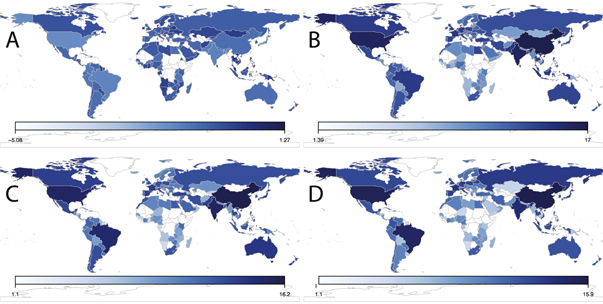
Figure 1. World maps for trade openness and nutrient use in 2006. National level trade openness (A), nitrogen use (B), phosphate use (C), and potash use (D) are shown. Note that the log of each variable is provided.
Download figure:
Standard image High-resolution imageBilateral trade: data on bilateral trade are collected from the International Monetary Fund (IMF) Direction of Trade Statistics (DOTS) (International Monetary Fund, Direction of Trade Statistics (DOTS), 2015). DOTS provides bilateral trade in value [$]. Annual data are available from 1947–1960, with monthly and quarterly data availability beginning in 1960.
Nutrient use: data on the nutrient use of nations are collected from the Food and Agriculture Organization of the United Nations Statistics Division (FAOSTAT) (FAOSTAT 2018). Specifically, we collect data on the total nitrogen (N), phosphate (P2O5), and potash (K2O) from all fertilizer products. Potash is any of various mined and manufactured salts that contain potassium in water-soluble form. Inorganic phosphates are mined to obtain phosphorus for use in agriculture and industry. National nutrient use data is provided for total nutrient use in agriculture [tonnes] and average nutrient use per area of cropland (kg ha−1). We collect this data at the county-year level from 2002–2014. Nutrient use for the year 2006 is mapped in figures 1(B)–(D).
Geography: we collect many geographic variables and country characteristics. We collect information on national area, landlocked dummy variable, border dummy variable, and the distance between pairs of countries from the GeoDist database (Mayer and Zignago 2011). We collect latitude, monthly average precipitation, and monthly average temperature from the World Bank data portal (World Bank 2015). We take the average of monthly precipitation and temperature to get the annual average. We collect total population (thousands) from United Nations Population Division (United Nations Population Division 2015). We collect capital stock at current PPPs (in mil. 2011 US$) from Feenstra et al (2015).
Trade agreements: information on World Trade Organization (WTO) accessions and regional trade agreements (RTAs) are also collected. Data on WTO accessions are provided by WTO accessions (2018) and a list of all RTAs in force are available from the Regional Trade Agreements Information System (RTA-IS) (2018). The RTA-IS is a database of the WTO that tracks RTAs beginning in 1948. The WTO accessions provide the year a country become a member of the WTO. The Accessions Intelligence Portal of the WTO contains information on on-going and completed WTO accessions since 1995. Thus, we calculate the WTO dummy which indicates whether a country is a member of the WTO in a given year. For each RTA, information is available on the date that the RTA came into force and the country signatories to the RTA. Thus, we calculate the RTA dummy which indicates whether two countries are in a RTA in a given year.
2.2. IV method
To isolate the causal impact of trade openness on nutrient use, we use an 'IV' in a 'two-stage least squares' approach (Angrist and Pischke 2009, Wooldridge 2010). For this method, we must identify a variable that is (1) strongly correlated with trade openness and (2) uncorrelated with any unobservable determinants of nutrient use. Such a variable is known as an 'instrument'. In the 'first stage' we regress the endogenous variable on the IV and a set of control variables. It is important that the IV should only affect nutrient use through the endogenous variable (openness in our case). In the 'second stage', the predicted value of the endogenous variable from the first stage is used as the independent variable to obtain a causal estimate.
We extend the IV approach employed by Frankel and Romer (1999) to an unbalanced panel of countries from 2002–2014. In this way, we use geographical variables to instrument for trade between nations. Now, we additionally incorporate time series information on the RTAs between nations as well as accession into the WTO. It is important to note that international trade negotiations in the context of the General Agreement on Tariffs and Trade and now the WTO have been focused primarily on the manufacturing sector since its inception. In fact, the last multilateral trade round (the Doha Round), that started in 2001 and was intended to focus on agriculture (and development), never came to a close, see Irwin (2009). This means that time-varying trade agreements and policies may not impact the agricultural sector as much as non-agricultural sectors of the economy, making them suitable instruments for openness in the analysis of nutrient use that is primarily stemming from a country's agricultural sector. Note that the panel IV approach enables us to include country and year fixed effects and to capture unobservable heterogeneity that is often left uncontrolled for in a cross section and gives way to bias in the estimation. We present two versions of our analysis. In version 1, we apply an IV based on geographical factors and changing trade policies to panel data. In version 2, we additionally control for the comparative advantage of countries to determine if trade openness interacts with countries differently when this is accounted for.
2.2.1. Version 1
The IV procedure is provided in equations (1) and (2). The first stage for the panel is provided in equation (1). In equation (1), the endogenous variable, i.e. the real trade openness for country c in year t, is regressed on the constructed trade openness variable for country c in year t ( ) and control variables,
  . The control variables are log of area per person
  , log of capital stock per person
  , log of population
  , precipitation prct, and temperature tasct. The second stage is provided in equation (2). In equation (2), log nutrient use for country c in year t (Uct) is regressed on predicted values of real trade openness for country c in year t, denoted as
  , and all the time-varying controls. It is critical that both equations (1) and (2) contain the same set of controls.

Note that equations (1) and (2) include country- and year-fixed effects (αc, αt) to control for unobserved heterogeneity. uct is the error term.
To construct an instrument in the panel context we add the interaction terms of distance and population to our instrument. This is because population does change in time, albeit slowly. Additionally, we incorporate changes in trade policy within our study time period. To do this, we include two indicator variables. The first indicator is wtoct and will be equal to one if country c is part of the WTO in a given year t (and zero otherwise). The second indicator is rtaijt and will be equal to one in case both trading countries (i and j) are part of a common RTA in a given year t (and zero otherwise).
To specify, the log transform of the bilateral trade share in a given year t is estimated as:
The instrument for trade openness for country i in year t is constructed by summing the estimated bilateral trade share in year t between country i and all other countries:

Note that this is the constructed trade openness that is used as the independent variable in equation (1).
2.2.2. Version 2
We also run a version of our analysis with interaction terms between openness and measures of countries' comparative advantage. The net impact of trade openness on a country's nutrient use should vary across countries. As countries open up to trade, they are no longer limited to producing whatever is wanted domestically, and trade theory predicts that they will specialize. Countries that have a comparative advantage in producing agricultural goods will produce more in agriculture and export in that sector. Complementing those exports, such countries will import goods they are not as good at producing from other countries (Feenstra 2015). Hence, we would expect that whether a country is prone to export or import in agricultural goods will affect its nutrient use differently. In the first case, more openness will give way to more exports that will increase overall nutrient use. In the second case, more openness should trigger more imports in agriculture. To capture how the impact of openness may vary by countries according to their comparative advantage of countries, we interact our openness measure with measures of countries' comparative advantage.
In particular, we include interaction terms of openness and resource endowment measures that are meant to capture the more likely export or import orientation of a country. Specifically, we include area per person A/P to capture the comparative advantage of a country to agricultural trade and the capital stock per person ck/P is included to capture the comparative advantage of countries to manufacturing trade. As countries open up to trade, their pattern of production is expected to shift in line with their comparative advantage. Countries with respectively more area per person A/P or capital stock per person ck/P are prone to have more of a comparative advantage in, respectively, agricultural production or manufacturing. Hence, the impact of more trade openness on nutrients that are most directly associated with agricultural production may well depend on whether a country is prone to export agricultural commodities or not, which could amplify or mitigate the level of nutrient use.
To properly capture the impact of the interacted variables, both A/P and ck/P will need to independently enter the regression on the right hand side. To specify, we use the constructed trade openness term ( ) and the two interaction terms (
 ,
,  ) to instrument for the three endogenous variables, i.e. the real trade openness (Tct) and the two interaction terms (
 ,
,  ). The control variables X are the same as in equations (1) and (2). As in equations (1) and (2), we control for country- and year-fixed effects. The first stages are in equations (5)–(7), and the second stage is in equation (8)


While we have no prior expectations about the impact of openness, we would expect a positive coefficient on the interaction term between openness and A/P, especially for the level of nutrient use. Indeed, we would expect that more A/P (i.e. more potential to produce agricultural output and exports) and more openness would reinforce each other. Alternatively, we would expect a negative coefficient on the interaction term of openness and ck/P for the level of nutrient use, to the extent that more ck/P gives way to more manufacturing (less agricultural) production and exports. Note that we have no clear prior expectation on the impact of openness as such and its interactions on the nutrient intensity (nutrient use per area). Openness could give way to an increase of fertilizer use, or (best case scenario), improvement in nutrient best management practices that lead to reductions in nutrient use.
In sum, in version one we will study the impact of openness as such on nutrient use without explicitly accounting for the comparative advantage of a country to produce agriculture (i.e. the nutrient using economic sector). Since nutrient use is directly tied to a specific sector of the economy (agriculture), a country's export or import capacity in agriculture can amplify or mitigate the impact of openness to trade on its nutrient use. Therefore, we bring in two interaction terms in version two of our specification to account for comparative advantage to trade. We interact openness, on the one hand, with a country's capital per person and, on the other hand, with its land area per person. These two variables influence a country's comparative advantage to produce in different economic sectors. We expect, respectively, a negative and a positive coefficient for the two variables: the more open and the more capital abundant it is, the more its ability to export in agriculture shrinks, and the less nutrient use one expects. We expect a positive coefficient on the interaction between land abundance and openness, so that more openness is amplified by a shift towards agriculture which should positively impact nutrient use.
2.2.3. Instrument quality
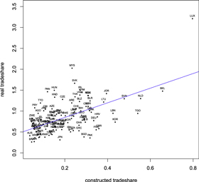
Our instrument (1) must be highly correlated with actual trade openness (i.e. the instrumented variable) and (2) must not be correlated with other drivers of nutrient use in the error term. To check the first condition, we evaluate the relationship between the instrument (constructed trade openness,  ) and the instrumented variable (actual trade openness). We plot the relationship between actual and constructed trade openness for each country in figure 2. This relationship is roughly linear and increasing, providing evidence that the first assumption for a high quality instrument is satisfied. We use the Kleibergen-Paap statistic rk Wald F statistic ('First stage F-statistic' ) to quantify the relationship between the actual and constructed trade share. The first stage F statistic is almost always greater than 10, which is the rule-of-thumb value for strong instruments. These results indicate that our instrument is not weak.
Figure 2. Real tradeshare versus constructed tradeshare. Note that this graph is for the year 2006 and all other years are similar.
Download figure:
Standard image High-resolution image
To avoid (2) we include controls. Note that, in addition to the panel analysis, we also perform the cross-sectional regression. We do this so that our results for the cross section can be compared with existing literature, which is primarily for the cross-section, by the interested reader. All of our cross-sectional results are presented in the supporting information (available online at stacks.iop.org/ERL/13/124016/mmedia). In the cross section, we control for land area (A), population (P), latitude (lat), precipitation (pr), and temperature (tas), which may potentially be correlated with the distance measures introduced by Frankel and Romer (1999). The advantage of our panel regression is that we can include country and year dummies that will capture unobserved country and year specific factors that drive the left-hand side variable. To be consistent, we include the same time-varying control variables in the panel analysis as in the cross-section. This means that we include all of the same controls in the panel analysis with the exception of latitude, as it does not vary with time.
3. Results and discussion
Here, we present and discuss results on the relationship between trade openness and the nutrient use of nations. Visually, it is not clear how trade openness and the national use of nutrients are correlated (i.e. compare figure 1(A) with (B)–(D)).
3.1. Version 1
The panel estimates for all outcome variable for version 1 are presented in table 2. We also present OLS coefficients in table 2(A) as a point of comparison. Note that the OLS panel regression equation is given by:
where U is nutrient use, T is trade openness, and X are the control variables. c is a country index, t is a year index, and υ is the error term. The control variables are the same as in equations (1) and (2). The coefficient of interest is d1, which indicates the correlational relationship between trade openness and nutrient use.
Table 2. Panels results for OLS and IV coefficients for all nutrient outcome variables. Note that these panel results correspond to version 1 (without interaction terms).
| log(N) | log(P) | log(K) | log(N per Area) | log(P per Area) | log(K per Area) | |
|---|---|---|---|---|---|---|
| (1) | (2) | (3) | (4) | (5) | (6) | |
| A: OLS | ||||||
| openness_real | −0.247
|
−1.019
|
−0.430
|
−0.254
|
−1.024
|
−0.437
|
| (0.100) | (0.175) | (0.176) | (0.098) | (0.174) | (0.176) | |
| B: IV (second stage) | ||||||
| openness_real | −0.61 | −1.49 | −1.32 | −0.85 | −1.74 | −1.55 |
| (0.85) | (1.46) | (1.47) | (0.83) | (1.45) | (1.47) | |
| C: IV (first stage) | ||||||
| F-stat | 15.9*** | 15.9*** | 15.9*** | 15.9*** | 15.9*** | 15.9*** |
| n_obs | 1027 | 1027 | 1027 | 1027 | 1027 | 1027 |
*p < 0.1;  p < 0.05;
  p < 0.01.
In table 2(A) all OLS coefficients are statistically significant and negative. OLS coefficients are statistically significant for both total nutrient use and nutrient use per area. However, these OLS coefficients are subject to endogeneity concerns, which is why we run the IV analysis. The IV first stage results are shown in table 2(C). The F-stat for the first stage is always greater than 10 and statistically significant. This indicates that our instrument for trade is not weak. The IV second stage results are presented in table 2(B). The IV coefficients are all negative across the board but statistically insignificant. Our OLS specification indicates that trade openness leads to a reduction in nutrient use, while our IV specification shows that there is no statistically significant impact of trade openness on nutrient use.
3.2. Version 2
Version 2 panel results are presented in table 3. Again, we compare our IV estimates with an OLS panel regression, now given by:

where all variables are defined as before and again the control variables are the same as in equations (1) and (2). The interaction terms Z1 and Z2 are included in this specification. Now, when we interact openness with A/P and ck/P the OLS coefficients are mostly insignificant except for the case of nitrogen (refer to table 3(A)). The interaction between openness and land per person is positive and significant, and the interaction with capital per person is insignificant or negative and significant for log(K) and log(K per Area). As noted, there are endogeneity concerns for the OLS estimates, which is why we instrument.
Table 3. Panels results for OLS and IV coefficients for all nutrient outcome variables. Note that these panel results correspond to version 2 (with interaction terms).
| log(N) | log(P) | log(K) | log(N per Area) | log(P per Area) | log(K per Area) | |
|---|---|---|---|---|---|---|
| (1) | (2) | (3) | (4) | (5) | (6) | |
| A: OLS | ||||||
| openness_real | 0.857* | 0.944 | 1.041 | 0.775 | 0.856 | 0.957 |
| (0.500) | (0.875) | (0.872) | (0.489) | (0.867) | (0.875) | |
| openness_real:log(lperP) |

|

|

|

|

|

|
| (0.091) | (0.159) | (0.159) | (0.089) | (0.158) | (0.159) | |
| openness_real:log(ckperP) | −0.008 | 0.039 | −0.184
|
−0.001 | 0.044 | −0.176
|
| (0.050) | (0.087) | (0.087) | (0.049) | (0.087) | (0.088) | |
| B: IV (second stage) | ||||||
| openness_real | 1.53 | −6.62 * | −4.66 | 1.04 | −7.14 * | −5.15 |
| (2.44) | (3.96) | (3.98) | (2.36) | (3.91) | (3.96) | |
| openness_real:log(lperP) | 0.4 | −0.74 | −0.44 | 0.36 | −0.78 | −0.48 |
| (0.44) | (0.7) | (0.71) | (0.42) | (0.7) | (0.71) | |
| openness_real:log(ckperP) | −0.52 * | −0.58 | −1.18 ** | −0.56 * | −0.62 | −1.21 ** |
| (0.3) | (0.48) | (0.49) | (0.29) | (0.48) | (0.49) | |
| C: IV (first stage) | ||||||
| F-stat (openness_real) | 11.54*** | 11.54*** | 11.54*** | 11.54*** | 11.54*** | 11.54*** |
| F-stat (openness_real:log(lperP)) | 13.15*** | 13.15*** | 13.15*** | 13.15*** | 13.15*** | 13.15*** |
| F-stat (openness_real:log(ckperP)) | 15.68*** | 15.68*** | 15.68*** | 15.68*** | 15.68*** | 15.68*** |
| n_obs | 1027 | 1027 | 1027 | 1027 | 1027 | 1027 |
*p < 0.1;  p < 0.05;
  p < 0.01.
In a few cases, when we include the interaction terms to account for comparative advantage, the IV coefficients become statistically significant (refer to log(P) and log(P per Area) in table 3(B)). The interaction of openness with ck/P tends to be mostly negative and significant for log(N), log(K), log(N per Area), and log(K per Area), which is in line with our expectations. Note that the interaction with land/P is positive but insignificant. On balance these are quite intuitive results. They show that if there is an effect of openness on nutrient use, it tends to be negative and to move in line with what one would expect in terms of comparative advantage. Countries that become more open and have an ever stronger comparative advantage in manufacturing (not agriculture) tend to see the level of their nutrient use decrease. Interestingly, this also translates into a decrease in the nutrient use per area as well. Note that an alternative explanation of this effect is also possible, due to the high correlation between ck/P and per capita GDP. As countries become richer (higher per capita GDP), they tend to care more about environmental issues, and tend to introduce environmentally friendly policies, as suggested by Antweiler et al (2001).
Thus, the IV method, which more closely estimates the causal impact of trade on an outcome of interest, indicates that trade openness does not significantly impact nutrient use, or reduces it. In sum, our IV panel estimates that incorporate variation over time, and that allow us to better control for unobserved heterogeneity with fixed effects, tend to be either insignificant or negative. When we include the interaction terms to account for the comparative advantage of a country, we see that openness reduces nutrient use especially as countries become more capital abundant. This could be explained by countries shifting their economies away from agriculture, or, alternatively, since capital abundance is correlated with per capita GDP, these countries may start caring more about environmental issues.
4. Conclusion
This paper contributed to the debate over globalization and the environment. The major question that this paper addressed is: What is the impact of trade openness on national nutrient use? Our results suggest that trade openness does not significantly impact the nutrient use of nations, or, if anything, reduces it. This is in line with previous research that shows that trade openness does not have a negative impact on the environment (Antweiler et al 2001, Frankel and Rose 2005). To reach this conclusion we employed the IV method, which explicitly addresses endogeneity in order to evaluate causal relationships that exist in data (Angrist and Pischke 2009). We build upon the method introduced by Frankel and Romer (1999), which is based upon the geographical features of nations, by performing a panel analysis to take advantage of time series variation and account for unobservable heterogeneity between countries. We used time-varying information on trade agreements to incorporate time variation in our instrument for trade.
Additionally, we determine whether those countries that specialize in agriculture (the nutrient using sector) are impacted by trade openness differently from countries with a comparative advantage in manufacturing. Our findings suggest that trade openness does not significantly impact nutrient use, or reduces it as countries become more capital abundant. This finding can be explained by countries shifting their economies away from agriculture, or, alternatively since capital abundance is correlated with per capita GDP, as countries become more affluent, they start demanding higher environmental quality.
This work contributes to a body of literature that generally finds that trade does not negatively impact the environment, making it of interest to the science and policy communities. This paper empirically determined that trade does not have unintended consequences for the quantity of nutrients that we use to produce our food. Recent work has presented a theoretical model of water and trade (Dang et al 2018) that is consistent with empirical findings on the relationship between trade and water use (Kagohashi et al 2015, Dang and Konar 2016). Now, we suggest there is a need for a similar model to be developed to explain the mechanistic relationship between trade and nutrient use. We suggest that future modeling efforts could aim to be consistent with the empirical findings presented in this paper. Additionally, future empirical work could examine how trade openness impacts agricultural decision making more broadly, as this is the main channel through which nutrient use is impacted.
Acknowledgments
This material is based upon work supported by the National Science Foundation Grant No. ACI-1639529 ('INFEWS/T1: Mesoscale Data Fusion to Map and Model the US Food, Energy, and Water (FEW) System') and EAR-1534544 ('Hazards SEES: Understanding Cross-Scale Interactions of Trade and Food Policy to Improve Resilience to Drought Risk'). Any opinions, findings, and conclusions or recommendations expressed in this material are those of the author(s) and do not necessarily reflect the views of the National Science Foundation. All data sources are detailed in table 1 and are publicly accessible. We gratefully acknowledge these sources, without which this work would not be possible.