


Abstract
The Southern Hemisphere (SH) zonal-mean circulation change in response to Antarctic ozone depletion is re-visited by examining a set of the latest model simulations archived for the Chemistry-Climate Model Initiative (CCMI) project. All models reasonably well reproduce Antarctic ozone depletion in the late 20th century. The related SH-summer circulation changes, such as a poleward intensification of westerly jet and a poleward expansion of the Hadley cell, are also well captured. All experiments exhibit quantitatively the same multi-model mean trend, irrespective of whether the ocean is coupled or prescribed. Results are also quantitatively similar to those derived from the Coupled Model Intercomparison Project phase 5 (CMIP5) high-top model simulations in which the stratospheric ozone is mostly prescribed with monthly- and zonally-averaged values. These results suggest that the ozone-hole-induced SH-summer circulation changes are robust across the models irrespective of the specific chemistry-atmosphere-ocean coupling.
Export citation and abstract BibTeX RIS

Original content from this work may be used under the terms of the Creative Commons Attribution 3.0 licence.
Any further distribution of this work must maintain attribution to the author(s) and the title of the work, journal citation and DOI.
1. Introduction
The Southern Hemisphere (SH) general circulation underwent distinct changes in the late 20th century. Among others, the westerly jet shifted poleward (Chen and Held 2007, Swart et al 2015), often represented by the positive trend of the southern annular mode index. The poleward edge of the Hadley cell also shifted poleward (Hu and Fu 2007, Davis and Rosenlof 2012, Garfinkel et al 2015), implying a widening of the Hadley cell. In response to these changes, SH surface climate variables such as surface air temperature and precipitation also changed significantly (Gillett et al 2006, Thompson et al 2011, Gonzalez et al 2014).
Simultaneous with these changes, Antarctic ozone concentrations sharply decreased due to the emission of ozone depleting substances (Solomon 1999). In an attempt to substantiate the causal link between the Antarctic ozone depletion and SH tropospheric and surface climate changes, multiple studies have performed climate model simulations with and without ozone depletion (e.g. Polvani et al 2011, McLandress et al 2011, Waugh et al 2015). A common feature of these studies is that a rapid decline of the austral-spring ozone concentrations in the lower stratosphere tends to force the austral-summer jet and Hadley cell to shift poleward. More importantly, these ozone-hole-induced circulation changes in austral summer are much stronger than the greenhouse-gas-induced ones. Although the detailed mechanism(s) remains to be determined, similar results are also seen in multi-model ensembles, e.g. the Coupled Model Intercomparison Project (CMIP) phase 3 or 5 (Meehl et al 2007, Taylor et al 2012) and the Chemistry-Climate Model Validation activity 2 (CCMVal2; Eyring et al 2010), stressing that Antarctic ozone hole has played a predominant role in the austral-summer SH circulation changes in the late 20th century (Son et al 2009, Min and Son 2013, Gerber and Son 2014, Tao et al 2016, Choi et al 2018).
Only two studies do not conclude that ozone depletion dominated historical SH-summer circulation changes (Staten et al 2012, Quan et al 2014), and this can be partly traced back to the methodology used in their studies (Waugh et al 2015). It can be also influenced by the different sea surface temperature (SST) forcings (Staten et al 2012). However, the influence of SST variation on 20th century SH circulation changes is likely much weaker than the ozone-hole-induced ones (Waugh et al 2015). SST variations become important only after 2000 when ozone concentrations plateaued (Garfinkel et al 2015).
While the poleward intensification of the SH-summer jet in response to Antarctic ozone depletion is reasonably well simulated by most climate models, its magnitude differs substantially among models (e.g. Son et al 2009, Gerber and Son 2014). This inter-model spread could be caused by several, likely complementary factors. The most immediate factor is the precise manner in which stratospheric ozone is imposed. While some models interactively simulate stratospheric chemistry and hence simulate an ozone hole with a three-dimensional structure that varies consistently with dynamical fields (e.g. CCMVal2 models), others simply prescribe stratospheric ozone using an off-line ozone dataset (e.g. CMIP3 and most CMIP5 models). Modeling studies have shown that the formers tend to simulate stronger tropospheric trends than the latters (Gillett et al 2009, Waugh et al 2009, Li et al 2016). This difference is caused not only by the realism of the ozone forcing but also by model biases in the simulation of the stratospheric polar vortex. Most CCMVal2 models, for example, suffer from a delayed break-up of the stratospheric polar vortex (Butchart et al 2011), and this bias can lead to an overestimate of the ozone-hole effect (Lin et al 2017). The ozone-hole-induced circulation change can be also sensitive to the temporal resolution and spatial structure of prescribed ozone: models prescribing daily and zonally asymmetric ozone often show stronger circulation changes than those forced by monthly and zonally-mean ozone (e.g. Crook et al 2008, Neely et al 2014).
However, the above sensitivities, which are mostly based on single model experiments with varying stratospheric ozone, do not explain differences between multi-model ensembles. For example, differences in the SH-summer circulation changes between CMIP3 simulations (where monthly- and zonally-averaged ozone is prescribed) and CCMVal2 simulations (where stratospheric ozone is fully interactive) are only minor (see figure 4 of Gerber et al 2012). Seviour et al (2017) also documented no systematic differences between model simulations with and without interactive ozone chemistry, and instead suggested that differences among simulations could reflect natural variability in the tropospheric circulation.
The SH-summer circulation changes could also be sensitive to surface boundary conditions. A poleward intensification of the jet can lead to cooler SST anomalies in high-latitudes but warm SST anomalies in mid-latitudes through the wind-driven meridional overturning circulation (Sigmond and Fyfe 2010, Thompson et al 2011). This SST change is then modified by a time-delayed deep ocean circulation change (Ferreira et al 2015, Seviour et al 2016). The net SST change differs substantially among the models (Ferreira et al 2015), introducing an uncertainty in the SH circulation change. Note that most CCMVal2 models were not configured with a coupled ocean (Morgenstern et al 2010), and hence the SST and sea ice concentration (SIC) did not evolve in a physically consistent manner with the overlying atmosphere.
Table 1. List of CCMI models used in this study. Each model's acronym can be found in Morgenstern et al (2017). The model resolution is indicated in terms of horizontal resolution (longitude × latitude) and the number of vertical levels. Models with only stratospheric chemistry are denoted with 'Strat', while those incorporating both stratospheric and tropospheric chemistry are denoted with 'Strat-Trop'. Models with relatively simple tropospheric chemistry are separately denoted with 'Strat-sTrop'. In the fourth column, 'Coupled' indicates the model in which the ocean is coupled in CCMI-C2 run.
| Model | Resolution | Chemistry | CCMI-C2 ocean |
|---|---|---|---|
| ACCESS-CCM | 3.75° × 2.5° L60 | Strat-Trop | Uncoupled |
| CCSRNIES-MIROC3.2 | T42 L34 | Strat | Uncoupled |
| CESM1-CAM4Chem | 1.9° × 2.5° L26 | Strat-Trop | Coupled |
| CESM1-WACCM | 1.9° × 2.5° L66 | Strat-Trop | Coupled |
| CMAM | T47 L71 | Strat-Trop | Uncoupled |
| CNRM-CM5.3 | T63 L60 | Strat | Uncoupled |
| EMAC-L47MA | T42 L47 | Strat-Trop | Coupled |
| EMAC-L90MA | T42 L90 | Strat-Trop | Uncoupled |
| GEOSCCM | 2° × 2° L72 | Strat-Trop | Uncoupled |
| HadGEM3-ES | 1.875° × 1.25° L85 | Strat-Trop | Coupled |
| MRI-ESM1r1 | TL 159 L80 | Strat-Trop | Coupled |
| NIWA-UKCA | 3.75° × 2.5° L60 | Strat-Trop | Coupled |
| SOCOL3 | T42 L39 | Strat-sTrop | Uncoupled |
| UMSLIMCAT | 3.75° × 2.5° L64 | Strat | Uncoupled |
| UMUKCA-UCAM | N48 L60 | Strat-sTrop | Uncoupled |
The purpose of the present study is to re-assess the ozone-hole-induced tropospheric circulation changes by examining recent CCM simulations that were performed for the CCM Initiative (CCMI) project (Eyring et al 2013b, Morgenstern et al 2017). We address whether up-to-date CCMs, which have coupled ocean and more comprehensive chemistry, can represent a more realistic jet and its long-term trend compared with CCMVal2 simulations (Son et al 2010). Another purpose is to re-evaluate the importance of interactive ozone chemistry and a coupled ocean. This issue was recently addressed by Seviour et al (2017), who performed time-slice experiments with varying stratospheric ozone forcing with and without a coupled ocean, but is extended in this study to multi-model transient simulations. For this purpose, the CCMI model simulations with and without a coupled ocean are directly compared. The multi-model mean trend of the CCMI simulations is also compared with that of the CMIP5 simulations.
Here it should be stated that the models analyzed in this study are not solely driven by ozone depletion. Other forcings, such as increasing greenhouse gas concentrations and anthropogenic aerosol loadings, are also included. But, based on previous studies (e.g. Polvani et al 2011, Waugh et al 2015), it is assumed that the SH-summer circulation changes in the late 20th century are mostly driven by Antarctic ozone depletion.
2. CCMI and CMIP5 datasets
The CCMI was jointly launched by the International Global Atmospheric Chemistry (IGAC) and the Stratosphere-troposphere Processes And their Role in Climate (SPARC) to better understand chemistry-climate interactions in the recent past and future climate (Eyring et al 2013b). This modeling effort is an extension of CCMVal2 (Eyring et al 2010), but utilizes up-to-date CCMs. The CCMI models used in this study are listed in table 1. All models that provide the reference simulations of the recent past and future climate are considered. Models with missing data or low resolution (coarser than T42 resolution) are excluded. As briefly described in table 1, tropospheric chemistry, in addition to stratospheric chemistry, is fully interactive in most models (Morgenstern et al 2017). This differs from most of the CCMVal2 models in which only stratospheric chemistry is interactive (Morgenstern et al 2010). More importantly, six CCMI models (i.e. CESM1-CAM4Chem, CESM1-WACCM, EMAC-L47MA, HadGEM3-ES, MRI-ESM1r1, and NIWA-UKCA) are integrated with a coupled ocean (Morgenstern et al 2017), enabling us to evaluate the role of chemistry-atmosphere-ocean coupling in SH climate change.
Two sets of CCMI simulations, i.e. REF-C1 and REF-C2, are investigated in this study (Eyring et al 2013b, Morgenstern et al 2017). The CCMI REF-C1 (hereafter referred to as CCMI-C1) experiment is a historical simulation, forced by observed SST/SIC. In contrast, the CCMI REF-C2 (hereafter CCMI-C2) experiment covers not only historical period but also future climate. This experiment is conducted either with a coupled ocean or with modeled SST/SIC taken from coupled model simulations (e.g. CMIP5). The one-to-one comparison of these two experiments thus allows us to quantify the importance of surface boundary conditions.
To identify the importance of interactive chemistry, CCMI simulations are also compared with CMIP5 historical simulations. Only the high-top CMIP5 models, which have a model top at 1 hPa or higher, are considered in this study (table 2). Most of them are forced by the SPARC ozone data or its modified version (Eyring et al 2013a). However, several models have fully interactive ozone chemistry and can be considered as CCMs (four models in table 2). In fact, two of them, i.e. CESM1-WACCM and MRI-ESM1, participated in the CCMI project. Not surprisingly, these models have quantitatively different ozone evolution from the SPARC ozone data. However, for simplicity, multi-model mean trends are constructed by averaging all CMIP5 high-top model simulations without consideration of the details of ozone chemistry. A comparison between the CMIP5 models with and without interactive chemistry is only briefly discussed.
Table 2. List of CMIP5 models used in this study. Only high-top models, that have a model top at 1 hPa and higher, are used. Models prescribing ozone depletion are denoted with 'Prescribed', while those incorporating semi-offline chemistry or fully interactive ozone chemistry are denoted with 'Semi-offline' or 'Strat-Trop', respectively. Note that, unlike CCMI models, all CMIP5 models are coupled with an ocean.
| Model | Resolution | Chemistry |
|---|---|---|
| CESM1-WACCM | 1.9° × 2.5° L66 | Strat-Trop |
| CMCC-CMS | T63 L95 | Prescribed |
| GFDL-CM3 | C48 L48 | Strat-Trop |
| HadGEM2-CC | N96 L38 | Prescribed |
| IPSL-CM5A-LR | 1.875° × 3.75° L39 | Semi-Offline |
| IPSL-CM5A-MR | 1.25° × 2.5° L39 | Semi-Offline |
| IPSL-CM5B-LR | 1.875° × 3.75° L39 | Semi-Offline |
| MIROC4h | T213 L56 | Prescribed |
| MIROC-ESM | T42 L80 | Prescribed |
| MIROC-ESM-CHEM | T42 L80 | Strat-Trop |
| MPI-ESM-LR | T63 L47 | Prescribed |
| MPI-ESM-MR | T63 L95 | Prescribed |
| MPI-ESM-P | T63 L47 | Prescribed |
| MRI-CGCM3 | T159 L48 | Prescribed |
| MRI-ESM1 | TL 159 L48 | Strat-Trop |
All analyses are conducted with the first ensemble member of each model. All model output is interpolated onto a common resolution of 2.5° latitude by 2.5° longitude and 31 pressure levels before computing linear trends. Although model output is available even in the 2000s, only the period of 1960–2000 when Antarctic ozone depletion is well defined is considered. Since the same analysis period has been used in the literature (Son et al 2010, Eyring et al 2013a, Gerber and Son 2014, Garfinkel et al 2015), this allows a direct comparison with previous studies.

Figure 1. Temporal evolution of September-November (SON) total column ozone (TCO) anomalies, integrated poleward of 60°S, from (a) CCMI-C1, (b) CCMI-C2 and (c) CMIP5 historical simulations. The anomaly is defined as the deviation from the 1980–2000 climatology of each model, and is slightly smoothed with a 1-2-1 filter. In (c), dashed lines denote the models with interactive chemistry. The models that use the same ozone data (e.g. three MPI-ESM models, CMCC-CMS, and HadGEM2-CC as described in Eyring et al 2013a) are indicated with same color. For reference, the observed TCO anomalies, derived from the Multi Sensor Re-analysis version 2 (MSR-2; Van der et al 2015) and the National Institute of Water and Atmospheric Research-Bodeker Scientific (NIWA-BS; Bodeker et al 2005) data sets, are superimposed with filled and open dots.
Download figure:
Standard image High-resolution image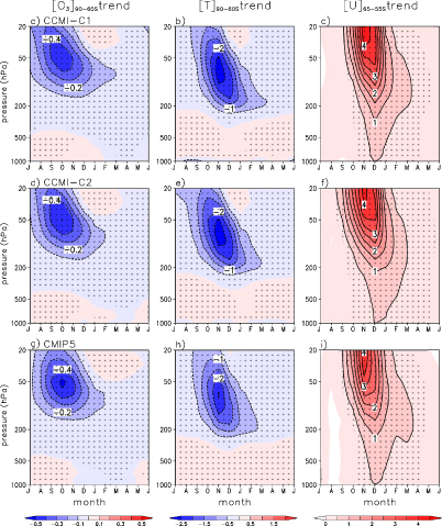
Figure 2. Multi-model mean trends of (left) monthly-mean polar-cap ozone concentration, (middle) temperature, and (right) mid-latitude zonal wind for the period of 1960–2000 for (top) CCMI-C1, (middle) CCMI-C2, and (bottom) CMIP5 historical simulations. Both ozone and temperature are integrated poleward of 60°S with area weighting, whereas zonal wind is averaged from 65°S–55°S. In all panels, x-axis starts from July and ends in June. Contour intervals are 0.1 ppmv/decade for ozone, 0.5 K decade−1 for temperature, and 0.5 m s−1/decade for zonal wind. The trends that are statistically significant at the 95% confidence level (based on Student's t-test) are dotted.
Download figure:
Standard image High-resolution image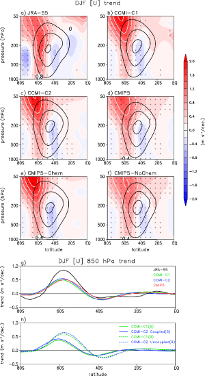
Figure 3. DJF zonal-mean zonal wind climatology (contour) and long-term trend for the period of 1960–2000 (shading) for (a) JRA-55, (b) CCMI-CI, (c) CCMI-C2, and (d) CMIP5 multi-model means. (e) and (f) Same as (d) but for the models with and without interactive chemistry. Contour interval of climatological wind is 10 m s−1 starting from 10 m s−1. The trends that are statistically significant at the 95% confidence level (based on Student's t-test) are dotted. Bottom panels show (g) 850 h Pa zonal wind trends from JRA-55 and model output and (h) sub-composite for the six models with a coupled ocean and the nine models where surface boundary conditions are prescribed (see table 1).
Download figure:
Standard image High-resolution image
Figure 4. The relationship of DJF jet-latitude trends (a) to ONDJ polar-stratospheric ozone trends and (b) to DJF Hadley-cell edge trends for the period of 1960–2000. The jet latitude is determined with 850 h Pa zonal-mean zonal wind, while polar-stratospheric ozone is defined by 100 h Pa ozone area-weighted from 60°S to the pole. Models that show statistically significant jet-latitude trends are denoted with light colored symbols, while those with insignificant trends are denoted with open symbols. The cross and filled symbols indicate the trends derived from JRA-55 and multi-model means. Correlation coefficient for each experiment is indicated in the parenthesis, following the experiment name, with an asterisk if the value is statistically significant at the 95 % confidence level based on Student's t-test. Bar graph in (c) shows the jet latitude trend difference between CCMI-C1 and CCMI-C2 simulations. When the difference is statistically significant at the 95% confidence level, it is filled.
Download figure:
Standard image High-resolution image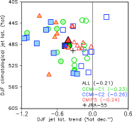
Figure 5. The relationship between DJF jet-latitude trends and climatological jet latitude. Overall format is same as in figure 4(a).
Download figure:
Standard image High-resolution image
3. Results
Figure 1 presents the evolution of September-November (SON) total column ozone (TCO) anomaly, area-weighted from 60°S to the pole, for each model. Here, the anomaly is defined as the deviation from the 1980–2000 climatology of each model. All models, i.e. CCMI-CI, CCMI-C2, and CMIP5 models, reasonably well reproduce a reduction in TCO as has been observed (Bodeker et al 2005, Van der et al 2015). The spatial distribution of the monthly-mean TCO and its seasonal cycle are also reasonably well captured (not shown). A comparison between figures 1(a) and (b) further reveals that, for each model, CCMI-C1 and CCMI-C2 simulations have a quantitatively similar TCO evolution (compare the same color on each panel). Since the two experiments differ mainly in surface boundary conditions (e.g. SST and SIC), this result may suggest that stratospheric ozone chemistry and transport is only weakly sensitive to the details of surface boundary conditions.
A pronounced inter-model spread, however, is evident especially in the 1960s and 1970s (figures 1(a) and (b)). This divergence among the models is similar to that seen in the CCMVal2 models (Austin et al 2010), and indicates that CCMs still have a large uncertainty in their simulation of Antarctic ozone. Unlike CCMI models, CMIP5 models show a quantitatively similar TCO evolution among the models (figure 1(c)). This is anticipated because most CMIP5 models are forced by the SPARC ozone data or its modified version. But, the CMIP5 models with interactive ozone chemistry also show a similar TCO evolution (see the dashed lines in figure 1(c)).
The vertical structure of polar ozone trends is illustrated in the first column of figure 2. The ozone depletion in the CCMI simulations is maximum at ~50 hPa in October. This is quantitatively similar to the one derived from the SPARC ozone data (e.g. figure 2(c)). The subtle differences between the experiments, such as a stronger upper-stratospheric ozone depletion in CCMI runs than in CMIP5 runs, are mostly insignificant.
The temperature response to the ozone depletion and the related stratospheric circulation change is shown in the middle column of figure 2. All experiments show significant cooling trend, centered at ~70 hPa, in November. This cooling trend extends from the middle stratosphere to the lower stratosphere with a maximum cooling at 20 hPa in October but at 200 hPa in December. Due to the thermal wind balance, a strong cooling in late spring is accompanied by a strengthening of the polar vortex (third column of figure 2). However this acceleration, which is a maximum in November, is not confined within the stratosphere but extends down into the troposphere. A statistically significant trend in the troposphere is particularly evident in December.
The temporal and vertical structure of polar ozone, temperature and mid-latitude wind trends, shown in figure 2, is remarkably similar to that of CCMVal2 simulations (figures 3(a)–(c) of Son et al 2010), indicating no major difference in multi-model mean trends between the CCMVal2 models and their updated versions. Such a similarity is also found in the December-February (DJF) zonal-mean zonal wind trends (figures 3(b)–(d)). For reference, the trend derived from the Japanese 55 year Reanalysis (JRA-55; Ebita et al 2011) is also displayed in figure 3(a). This data is chosen simply because it is the latest reanalysis dataset covering the analyzed period. All experiments show quantitatively a similar poleward intensification of westerly jet that resembles the reanalysis trend and the CMIP3/CCMVal2 trends (e.g. figure 4 of Gerber et al 2012). Note that CMIP5 models show a somewhat weak polar vortex change compared with CCMI models (figure 3(d)). This underestimation is mainly due to the models prescribing ozone depletion (figure 3(f)). Models with interactive and semi-offline chemistry (seven models listed in table 2) show essentially the same jet trend as CCMI models (figure 3(e)). However, regardless of polar vortex changes, two groups of CMIP5 models show quantitatively similar tropospheric circulation changes (compare figures 3(e) and (f)). This result is consistent with Eyring et al (2013a) who documented that CMIP5 models with interactive chemistry have larger inter-model spread and are not well separated from those without interactive chemistry (see their figures 10 and 11).
These results clearly suggest that the ozone-hole-induced tropospheric changes are not strongly sensitive to the coupled ocean and interactive chemistry when the multi-model mean trends are considered. This conclusion is supported by 850 hPa zonal wind trends (figure 3(g)). Their latitudinal distributions are almost identical among the model ensembles. The CCMI-C1 models with observed SST/SIC and the same models with a coupled ocean (CCMI-C2) are separately compared in figure 3(h) (blue and green solid lines; see table 1 for the six models with a coupled ocean). Likewise, CCMI-C1 models with observed SST/SIC and the same models with prescribed SST/SIC from the coupled models are compared (blue and green dashed lines). Each group again shows quantitatively the same multi-model mean trend, confirming the above conclusion.
All analyses so far are based on multi-model mean trends. Individual models, however, exhibit significantly different trends. For instance, the six CCMI-C2 runs with a coupled ocean and the other nine in figure 3(h) show non-negligible differences (compare blue solid and dashed lines). These differences can be partly traced back to different magnitudes of ozone depletion rather than different surface boundary conditions. Figure 4(a) shows the inter-model spread of DJF jet-latitude trends against polar-stratospheric ozone trends. Following previous studies (e.g. Son et al 2009), the jet latitude is determined as the latitude where a cubic fitted 850 h Pa zonal-mean zonal wind, around its maximum grid point and the two points either side, has the maximum. The lower-stratospheric ozone trends are quantified by the October–January (ONDJ) ozone trend at 100 hPa, area-weighted from 60°S to the pole, based on figure 2(a).
The CCMI simulations show a wide range of jet-latitude trends from ~1.2°/decade poleward shift to ~0.3°/decade equatorward shift (figure 4(a)). However, only half of them are statistically significant (light shaded symbols), indicating a large uncertainty in the simulated jet trends. Not surprisingly, the inter-model spread of the jet-latitude trends is highly correlated with that of the polar-stratospheric ozone trends. Their correlation is about 0.65 for both CCMI-C1 and CCMI-C2 simulations.
Figure 4(c) presents the one-to-one comparison between CCMI-C1 and CCMI-C2 simulations. The models with a coupled ocean in CCMI-C2 runs and those with observed SST/SIC in CCMI-C1 runs show no systematic differences (see purple bars; see also figure 3(h)). While three models show a weaker poleward jet shift when coupled to an ocean, the other three models show a stronger poleward jet shift. Moreover, none of these differences are statistically significant (see open bars). The CCMI-C2 runs with modeled SST/SIC and CCMI-C1 runs with observed SST/SIC also show no systematic differences (cyan bars). Although two models (i.e. EMAC-L90MA and SOCOL3) show statistically significant differences, they are opposite in sign. Although not presented, essentially the same results are found when the jet-latitude trends are normalized by the polar-stratospheric temperature trends. This confirms that the ozone-hole-induced SH-summer circulation changes are not strongly sensitive to the details of the surface boundary conditions (Seviour et al 2017).
All analyses are repeated for the Hadley cell edge. Here, the poleward edge of the Hadley cell is determined by the zero-crossing latitude of 500 h Pa mass stream function in the SH subtropics. During the austral summer, its trends are highly correlated with the jet-latitude trends (figure 4(b)). Their correlations across CCMI-C1, CCMI-C2, and CMIP5 runs are 0.87, 0.90, and 0.65, respectively. Consistent with previous studies (e.g. Son et al 2009), their ratio is close to 1-to-2 (see dashed line). Given this linear relationship, it is not surprising to find that overall results of the Hadley-cell changes are quite similar to the jet changes described above (not shown).
Previous ensembles of CCMs, such as CCMVal1, CCMVal2, and CMIP5 models with interactive chemistry, have suffered from biases in their mean state. Most CCMVal2 models, for instance, exhibit equatorward biases in the position of the climatological jet (see figure 10(b) of Son et al 2010). In terms of the multi-model mean, this bias is somewhat reduced in the CCMI simulations (see dark filled symbols in figure 5). However, compared to CCMVal2 models, the inter-model spread becomes larger with almost half of the models showing a poleward-biased climatological jet.
This bias has been related to different circulation responses to an identical forcing. Specifically, it has been proposed that models with an equatorward-biased jet tend to have a stronger jet response to the external forcing (Son et al 2010, Kidston and Gerber 2010). This argument, however, was questioned by recent studies (Simpson and Polvani 2016, Seviour et al 2017). Figure 5 displays the relationship between jet-latitude trends and climatological jet locations. Although there is a hint of a linear relationship (i.e. models with an equatorward-jet bias tend to have a stronger jet trend), all three model ensembles show statistically insignificant relationships. This result indicates that the dependency of the austral-summer jet trend on model mean bias, which was evident in CCMVal2 simulations (Son et al 2010), is not clear in CCMI models, supporting the recent studies of Simpson and Polvani (2016) and Seviour et al (2017).
4. Summary and discussion
This study updates previous studies based on the CCMVal2 simulations by examining the state-of-the-art CCMs that participated in the CCMI project (Eyring et al 2013b). Most of these models are successors to the CCMVal2 models with improved chemistry (especially in the troposphere). Six models are also coupled with an ocean. Both CCMI-C1 and CCMI-C2 simulations, which differ mainly in their sea surface temperature and sea ice conditions, exhibit quantitatively similar multi-model mean trends over the period of 1960–2000 that are characterized by the poleward intensification of the austral-summer jet. The resulting trends are also quantitatively similar to the ones derived from the CCMVal2 and CMIP5 high-top models. This result suggests that Antarctic ozone-hole-induced tropospheric changes are not strongly sensitive to the specific chemistry-atmosphere-ocean coupling (Seviour et al 2017). The sensitivity of the austral-summer circulation changes to the details of stratospheric ozone forcing, reported in previous studies (Gillett et al 2009, Waugh et al 2009, Staten et al 2012, Neely et al 2014, Li et al 2016), appears to be smaller than the inter-model spread (or uncertainty of the ozone-hole-induced tropospheric circulation change) and hence is not easily detectable.
All analyses shown in this study are based on only one ensemble member from each model. Although this allows a fair comparison among the models, it could make the result sensitive to the internal variability. To quantify the importance of internal variability, the analyses are repeated by considering all ensemble members. Here, multiple ensemble members (typically two or three) are available from six CCMI-C1 and seven CCMI-C2 models. Although not shown, overall results are not sensitive to the number of ensemble members. The multi-model mean trend based on only one ensemble member is quantitatively similar to the one derived from ensemble mean of each model.
Here we recall that all models analyzed in this study are forced not only by ozone depletion but also by all other external forcings such as increasing greenhouse gas concentrations and anthropogenic aerosol loadings. This implies that the austral-summer jet trends shown in this study are not solely driven by ozone depletion. Although it is well documented that ozone depletion is the major driver of historical SH-summer circulation change (e.g. Previdi and Polvani 2014), its relative importance against other forcings needs to be better quantified by examining the simulations with fixed ozone depleting substances (fODS) and fixed greenhouse gas (fGHG). Projected future circulation changes due to the anticipated ozone recovery also deserve further investigation.
Acknowledgments
We thank I Cionni for helpful discussion and sharing CMIP5 ozone dataset, the international modelling groups for making their simulations available for this analysis, the joint WCRP SPARC/IGAC CCMI for organizing and coordinating the model data analysis activity, and the British Atmospheric Data Centre (BADC) for collecting and archiving the CCMI model output. All datasets used in this study are available online: http://blogs.reading.ac.uk/ccmi/badc-data-access. The work by S-W Son and R Park was supported by Korea Ministry of Environment as 'Climate Change Correspondence Program'. C I Garfinkel was supported by the Israel Science Foundation (grant 1558/14). The work of N Butchart, S C Hardiman, and F M O'Connor was supported by the Joint UK BEIS/Defra Met Office Hadley Centre Climate Programme (GA01101) N Butchart and S C Hardiman were also supported by the European Commission's 7th Framework Programme, under grant agreement no. 603557, StratoClim project. F M O'Connor also acknowledges support from the Horizon 2020 European Union's Framework Programme for Research and Innovation Coordinated Research in Earth Systems and Climate: Experiments, kNowledge, Dissemination and Outreach (CRESCENDO) project under grant agreement no. 641816. The EMAC simulations were performed at the German Climate Computing Centre (DKRZ) through support from the Bundesministerium für Bildung und Forschung (BMBF). DKRZ and its scientific steering committee are gratefully acknowledged for providing the HPC and data archiving resources for the consortial project ESCiMo (Earth System Chemistry integrated Modelling). UMUKCA-UCAM model integrations were performed using the ARCHER UK National Supercomputing Service and the MONSooN system, a collaborative facility supplied under the Joint Weather and Climate Research Programme, which is a strategic partnership between the UK Met Office and the National Environment Research Council. O Morgenstern acknowledges funding by the New Zealand Royal Society Marsden Fund (grant 12-NIW-006) and by the Deep South National Science Challenge. The support by the NZ Government's Strategic Science Investment Fund (SSIF) through the NIWA programme CACV and the contribution of NeSI high-performance computing facilities are also acknowledged. New Zealand's national facilities are provided by the New Zealand eScience Infrastructure (NeSI) and funded jointly by NeSI's collaborator institutions and through the Ministry of Business, Innovation and Employment'sResearch Infrastructure programme. CCSRNIES-MIROC3.2 computations were performed on NIES computers (NEC–SX9/A(ECO), and supported by the Environment Research and Technology Development Fund (2–1709) of the Environmental Restoration and Conservation Agency. The CESM project was supported by the National Science Foundation and the Office of Science (BER) of the US Department of Energy. The National Center for Atmospheric Research is funded by the National Science Foundation. The CCM SOCOL model development and maintaining were supported by the Swiss National Science Foundation under grant agreement CRSII2_147659 (FUPSOL II). E Rozanov work was partially supported by the Swiss National Science Foundation under grants 200021_169241 (VEC) and 200020_163206 (SIMA).