

Abstract
High productivity temperate wetlands that accrete peat via belowground biomass (peatlands) may be managed for climate mitigation benefits due to their global distribution and notably negative emissions of atmospheric carbon dioxide (CO2) through rapid storage of carbon (C) in anoxic soils. Net emissions of additional greenhouse gases (GHG)—methane (CH4) and nitrous oxide (N2O)—are more difficult to predict and monitor due to fine-scale temporal and spatial variability, but can potentially reverse the climate mitigation benefits resulting from CO2 uptake. To support management decisions and modeling, we collected continuous 96 hour high frequency GHG flux data for CO2, CH4 and N2O at multiple scales—static chambers (1 Hz) and eddy covariance (10 Hz)—during peak productivity in a well-studied, impounded coastal peatland in California's Sacramento Delta with high annual rates of C fluxes, sequestering 2065 ± 150 g CO2 m−2 y−1 and emitting 64.5 ± 2.4 g CH4 m−2 y−1. Chambers (n = 6) showed strong spatial variability along a hydrologic gradient from inlet to interior plots. Daily (24 hour) net CO2 uptake (NEE) was highest near inlet locations and fell dramatically along the flowpath (−25 to −3.8 to +2.64 g CO2 m−2 d−1). In contrast, daily net CH4 flux increased along the flowpath (0.39 to 0.62 to 0.88 g CH4 m−2 d−1), such that sites of high daily CO2 uptake were sites of low CH4 emission. Distributed, continuous chamber data exposed five novel insights, and at least two important datagaps for wetland GHG management, including: (1) increasing dominance of CH4 ebullition fluxes (15%–32% of total) along the flowpath and (2) net negative N2O flux across all sites as measured during a 4 day period of peak biomass (−1.7 mg N2O m−2 d−1; 0.51 g CO2 eq m−2 d−1). The net negative emissions of re-established peat-accreting wetlands are notably high, but may be poorly estimated by models that do not consider within-wetland spatial variability due to water flowpaths.
Export citation and abstract BibTeX RIS

Original content from this work may be used under the terms of the Creative Commons Attribution 3.0 licence.
Any further distribution of this work must maintain attribution to the author(s) and the title of the work, journal citation and DOI.
Introduction
Due to high productivity and rising water tables via tidal connections, coastal vegetated wetlands generate long-term (millennial) autochtonous carbon (C) storage in peat and organic soils, largely through belowground biomass accretion (Drexler et al 2009, Morris et al 2016). Wetland management is often proposed as a means of coupling climate mitigation with climate adaptation (resilience to sea level rise; US White House Mid-Century Strategy for Deep Decarbonization 2016), as coastal wetland restoration often includes initial management for rapid accretion to reverse past subsidence due to drainage-induced oxidation and compaction (e.g. Deverel et al 2014, Baird et al 2017). Coastal peat-accreting wetlands are globally distributed (Frolking et al 2011), are subject to multiple human and climate stressors (e.g. Whittle and Gallego-Sala 2016), and once flooding is re-established, are capable of sequestering large amounts of carbon dioxide (CO2) annually through organic C accumulation (Miller et al 2008, Page et al 2009). However, as anoxic, carbon-rich environments, they can be significant emitters of methane (CH4) and nitrous oxide (N2O), especially at the freshwater end of the salinity gradient (Bridgham et al 2013). Identifying the optimal conditions for negative greenhouse gas (GHG) emission in managed coastal wetlands (i.e. maximal C uptake and minimal GHG release) requires finescale exploration of spatial and temporal patterns for sweet spots in the emissions balance.
GHG emissions from wetlands are difficult to map and quantify as their responses to environmental change can be conditional and non-linear. Although emergent patterns illustrate broad drivers such as temperature, water table, vegetation structure (e.g. Turetsky et al 2014, Yvon-Durocher et al 2014), biogeochemical feedbacks from vegetation in wetland soils are complex, preventing universal and direct correlations across varying spatial and temporal scales (e.g. Bhullar et al 2014). GHG emissions modeling thus requires an understanding of drivers most relevant to the scale of inquiry (Bridgham et al 2013). The issue of scale emerges in global inventory approaches as well, whereby bottom-up estimates can often exceed top-down inventory-based estimates of CH4 emissions (Saunois et al 2016). Wetland management to reduce global warming potentials (GWP) requires a process-based understanding of environmental drivers, and the extent to which they are subject to human manipulation. Studying the spatial variability of GHG fluxes within a single wetland complex (e.g. Waddington and Roulet 1996) can provide insight to process-based modeling, guidance on optimal wetland design for negative emissions, as well as guidance for verifying GWP (VCS 2015, ACR 2017) or sustained GWP (Neubauer and Megonigal 2015).
Because site measurements are often scaled to entire wetland complexes, we sought to test this assumption with concomitant datasets from eddy covariance (EC) and static chamber (SC) approaches. By comparing methods at different scales, we test the scaling relevance of spatial variability in net daily GHG budgets of CO2, CH4 and N2O exchange in a well-documented highly productive impounded coastal wetland of California's Sacramento–San Joaquin (SSJ) Delta. Alongside a long-running set of continuous annual EC flux stations (Anderson et al 2012, Knox et al 2015, Anderson et al 2016), we focused on the peak biomass period and collected high frequency (1 Hz) measurements in six chambers, two replicates at each of three evenly distributed, pre-established locations (piers) over a 96 hour period (four 24 hour days), to generate the data density needed to identify comparable rates among these spatially-explicit plots, and to identify pathways responsible for GHG flux along a hydrologic gradient. This data-dense, sub-habitat study identified novel processes regulating net GHG emissions, with important implications for model development and operational decision-making for wetlands being managed to optimize GHG removals.
Methods
Site
This study focuses on a well-documented, continuously flooded wetland complex established in 1997 to test the ability of managed wetlands to reverse subsidence in California's SSJ Delta (Miller et al 2008, Miller and Fujii 2010, Miller 2011, figure 1). The decadal trajectory of GHG emissions from the East Pond is described in Anderson et al (2016), and herein we describe atmospheric and hydrologic dynamics from the adjacent West Pond (figure 2). A historic intertidal peatland (Cowardin et al 1979, E2EM2) which is today a leveed and agriculturally-dominated island (polder), Twitchell Island has subsided nearly 8 meters over 150 years due to oxidation and compaction (Galloway et al 1999), with continuing rates of roughly 1.3 cm annually (Deverel et al 2016). Re-establishment of flooded conditions with slow freshwater flowthrough and dense colonization of emergent macrophytes (primarily Schoenoplectus acutus and Typha hybrid spp.) has generated conditions that halt subsidence and promote rapid peat accretion (Miller et al 2008), which may allow tidal reconnectivity and tidal marsh recovery within the century (Bates and Lund 2013). Decade-long monitoring with surface elevation tables (SETs) show that elevation gains have been orders of magnitude faster than that generated due to sea level rise (>400 v. <2 mm y−1 current SLR), with concomitant high rates of atmospheric C sequestration (10 year mean; 1 kg C m−2 y−1, Miller et al 2008). These rates of elevation gain in peat soils, as well as soil C accumulation, are among the highest documented in ecosystem C sequestration literature and are supported by the high rates of net uptake of atmospheric CO2 from gas flux measurements (Miller 2011, Knox et al 2015). Further, these rates comprise a spatially explicit range of peat accretion throughout the marsh, primarily along a hydrologic gradient from inlet to interior (Miller and Fujii 2011). As this site is not yet reconnected with tidal flows of surrounding channels, surface water levels are maintained with continuous water flow to be relatively constant (25 cm depth) with minimal lateral exports, since flow rates are balanced primarily by evaporation and transpiration (Fleck et al 2007).
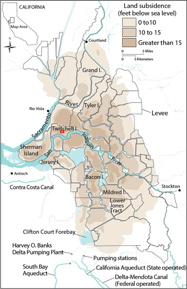
Figure 1. Location of California's Sacramento–San Joaquin Delta wetlands with map of current peat subsidence. Twitchell Island, in center left of map, is the research site and the study location and extent is identified by a small red box. Figure modified from Galloway et al 1999.
Download figure:
Standard image High-resolution image
Figure 2. Experimental distribution of gas flux measurement stations. Location of the eddy covariance (EC) flux tower along with the 80% and 90% footprints are indicated. Static chamber (SC) locations (n = 2 per Pier), indicated by letters A, B, and C, are arranged along a gradient of water flow, from the inlet (A), to more interior locations (B and then C), as the water generally flows slowly from inflow toward the outflows, with water levels maintained to account for evaporation and transpiration.
Download figure:
Standard image High-resolution imageChamber design
An intensive whole-plant-scale GHG flux study was conducted continuously over a 96 hour period, from August 29 through September 2, 2011, using a series of stationary chambers deployed in the West Pond (figure 2). Flux measurements were collected at three pre-established piers following the hydrologic gradient, with Pier A nearest the hydrologic inflow, Pier B located further west from the inflow, and Pier C farthest from the flowpath from inflow to outflow. Two identical chambers were erected on plots to customized heights at each of the three piers, using previously established PVC mounting attachments reported in Miller (2011).
Table 1 documents edaphic and structural conditions for each replicate chamber and site (vegetation characteristics, chamber volume and water levels). Species-specific vegetation biomass and leaf area were assessed by spectral assessments and published allometric relationships developed for the site (Miller and Fujii 2010, Byrd et al 2014). Diel patterns of physical conditions for water and air temperatures, PAR and barometric pressure within chambers were measured continuously (C1000/CFM, Campbell Scientific, Logan, UT, USA). The vegetation biomass gradient was the strongest structural difference among the sites, and followed the hydrological gradient with the tallest plants found at Pier A and heights decreasing to Pier C (e.g. aboveground biomass: 3.4–1.2 kg m2). Continuous water temperature data (figure 3, SI table 1 available at stacks.iop.org/ERL/13/045005/mmedia) illustrate diel and spatial patterns from inlet to interior sites that support a gradient of water quality documented by Miller and Fujii (2011) and indexed by cooling temperatures: higher temperatures and rapid turnover at the inlet (hourly), median turnover rates at the central location (daily) and low turnover rates at the interior (backwater) location (e.g. bi-weekly, Crepeau and Miller 2005). Inflowing waters from the Sacramento River are well mixed, slightly warmer than the shaded marsh surface, and consistently high in dissolved oxygen (>2 mg L−1) and low in nutrients such as nitrate (<0.5 mg L−1; USGS 2016, also see O'Connell et al 2014).

Figure 3. Record of continuous air and water temperatures at each Pier during the 96 hour study period, August 29 September 2 (1 Hz data).
Download figure:
Standard image High-resolution imageTable 1. Wetland structural conditions of replicate static chambers during the August–September 2011 sampling event. Max height is from base to tip of longest leaf, leaf area index (unitless) is a ratio of total leaf area to total surface area, Aboveground biomass is calculated with species-specific allometric equations on height, diameter and stem count, chamber volume is reported for internal dimensions, and water depth is reported as the average of initial and final conditions with n = 3 measurements at each time point. Maximal and minimal water temperatures are reported here, as extracted from continuous data reported in SI.
| Chamber | Dominant species | Max plant height | Leaf areaa allometric leaf/surface | Aboveground biomassb allometric | Chamber volume | Surface water depth—avg (n = 6) | Water temperature Max/Min |
|---|---|---|---|---|---|---|---|
| Rep | cm | m2/m2 | kgdw m−2 | m−3 | Cm | °C | |
| A1 | Schoenoplectus acutus | 329 | 6.2 | 2.8 | 1.83 | 20±3 | 20/18 |
| A2 | Schoenoplectus acutus | 335 | 8.1 | 3.4 | 1.79 | 19±3 | 20/18 |
| B1 | Schoenoplectus acutus/Typha hybrid spp. | 250 | 2.4 | 1.5 | 1.37 | 18±2 | 18/16 |
| B2 | Schoenoplectus acutus/Typha hybrid spp. | 245 | 2.2 | 1.2 | 1.39 | 17±3 | 18/16 |
| C1 | Typha hybrid spp./Schoenoplectus acutus | 249 | 2.3 | 1.3 | 1.37 | 17±2 | 18/16 |
| C2 | Typha hybrid spp./Schoenoplectus acutus | 234 | 2.1 | 1.2 | 1.33 | 18±1 | 18/16 |
As described by Miller (2011), the chambers (71 × 71 cm internal diameter) were enclosed by large transparent Mylar sleeves, which moved freely over the PVC structures and maintained consistent contact with the water's surface when lowered for chamber measurements. After testing replicability of sampling flow rates, fan speeds, and other deployment methods, chambers were deployed in a static mode, as non-steady-state, vented, flow-through systems. The air inside the chambers was cycled through a LGR Fast Greenhouse Gas Analyzer (FGGA, Los Gatos Research, Mountain View, CA, USA) in order to assess CH4 and CO2 concentrations as well as air temperature and water vapor (H2O) flux. Each of the three piers (two plots per pier) was staffed for >96 hours and equipped with its own computing station and sampling equipment: one FGGA (n = 3 total) and one manifold at each pier that allowed the air sampling stream to be alternated between the two replicate chambers in one-minute intervals for 16 min each hour beginning on the first minute of the hour. The two replicate chambers within a single site were thus sampled from a single calibrated platform of gas analysis equipment which was run continuously for over 100 hours. All gas and ancillary physical data was sampled at a rate of 1 Hz. The high data density required an evaluation of different advanced statistical procedures, which are described in SI appendix 1, and the alternative calculations presented in SI tables 3(a)–(f).
At the beginning of each hour (n = 96 hours reported), the Mylar sleeves were lowered synchronously across the first set of three chambers, and the sleeves were lowered on the second set of three chambers 1 minute later. In order to assure that the chamber environment was fully equilibrated through turbulent mixing, the first datapoints considered were 30–45 seconds after the lowering of Mylar sleeves, which remained lowered for the duration of the 16 m inute period. Briefly between each one-minute interval, ambient atmospheric air was cycled through the FGGA to provide a clear reference signal in the continuous record, in order to clearly distinguish gas streams from replicate chambers. At the end of each 16 minute sampling period, sleeves were raised and the chambers remained open until the next hour. In addition to CH4 and CO2, nitrous oxide (N2O) and carbon monoxide (CO) concentrations were analyzed over successive 24 hour periods, one day at each pier, using a lab-calibrated LGR N2O/CO Analyzer. When deployed at a given station, the LGR N2O/CO Analyzer was plumbed into the chamber manifold to concurrently sample the gas stream just after CH4 and CO2 measurements were taken with the FGGA. Method detection limits for gas concentrations of CO2, CH4, CO and N2O were 0.05 ppm, 0.8 ppb, 0.05 ppb, and 0.02 ppb, respectively.
Flux tower for cross-comparison with chambers
The eddy covariance (EC) method was used to measure 30 minute average fluxes of CO2 and CH4 at the ecosystem scale (Baldocchi et al 1988). The EC measurements reported herein were made at the site between 11 April 2011 and 16 April 2012 using equipment and methods reported in earlier publications (e.g. Knox et al 2015, Anderson et al 2016). In figure 2, we show the 80% and 90% analytical EC footprints during the period coinciding with the SC measurements. Flux footprint analysis suggests that EC flux measurements during the chamber campaign are likely most representative of fluxes measured from Pier A and least representative of fluxes measured from Pier C. Further details on EC methods and data quality are reported in SI appendix 2.
Table 2. Summary rates of gaseous flux (CO2, CH4, and N2O) in mass per m−2 for each of the six replicate chambers and eddy covariance during the August–September 2011 sampling event. Daytime peak, nighttime peak and daily mean ± standard deviation (n = 4 d) values are reported. For chamber measurements, methane (CH4) is reported for diffusive flux, ebullition flux (daily values only) and total flux. Eddy covariance flux data is reported for net CO2 and net CH4 only, with mean ± standard error. Error for N2O fluxes is reported only for all chambers (n = 6). Averages for all sites (All) assessed with all chamber data (n = 576 data points).
| CO2 | CO2 | CO2 | CH4 Diffusion | CH4 Diffusion | CH4 Diffusion | CH4 Ebullition | CH4 Total | CH4 Total | CH4 Total | N2O | N2O | N2O | |
|---|---|---|---|---|---|---|---|---|---|---|---|---|---|
| Daytime | Night | Daily (24 hr) | Daytime | Night | Daily (24 hr) | Daily (24 hr) | Daytime | Night | Daily (24 hr) | Daytime | Night | Daily (24 hr) | |
| g m−2 h−1 | g m−2 h−1 | g m−2 d−1 | g m−2 h−1 | g m−2 h−1 | g m−2 d−1 | g m−2 d−1 | g m−2 h−1 | g m−2 h−1 | g m−2 d−1 | g m−2 h−1 | g m−2 h−1 | g m−2 d−1 | |
| A1 | −3.37 ± 0.44 | 0.77 ± 0.09 | −16.68 ± 0.97 | 24.07 ± 1.13 | 9.47 ± 3.13 | 436.67 ± 13.33 | 70.00 ± 46.67 | 45.87 ± 16.67 | 9.47 ± 3.13 | 507.33 ± 51.33 | −0.29 | 0.11 | −1.93 |
| A2 | −4.44 ± 0.15 | 0.75 ± 0.04 | −32.82 ± 0.99 | 23.27 ± 5.33 | 10.33 ± 3.40 | 362.00 ± 42.00 | 66.00 ± 46.00 | 31.87 ± 9.33 | 11.60 ± 3.20 | 428.00 ± 84.67 | −0.26 | 0.02 | −1.96 |
| A Avg | −3.91 ± 0.18 | 0.75 ± 0.04 | −24.75 ± 0.95 | 23.67 ± 2.13 | 9.87 ± 1.73 | 398.67 ± 23.33 | 39.33 ± 23.33 | 38.80 ± 11.33 | 10.67 ± 19.33 | 467.33 ± 65.33 | −0.28 | 0.06 | 1.94 |
| 65.33B1 | −1.74 ± 0.18 | 1.25 ± 0.46 | −7.98 ± 1.58 | 33.87 ± 8.00 | 14.07 ± 1.27 | 492.00 ± 22.00 | 125.33 ± 38.00 | 43.40 ± 8.00 | 17.07 ± 3.53 | 617.33 ± 48.67 | −0.20 | 0.04 | −1.49 |
| B2 | −0.90 ± 0.28 | 1.01 ± 0.22 | −0.29 ± 2.57 | 28.53 ± 17.33 | 4.79 ± 1.27 | 285.33 ± 54.67 | 251.33 ± 97.33 | 80.00 ± 6.67 | 8.47 ± 0.33 | 536.67 ± 151.33 | −0.26 | 0.00 | −1.78 |
| B Avg | −1.28 ± 0.20 | 1.14 ± 0.33 | −3.83 ± 2.07 | 31.20 ± 12.00 | 9.47 ± 0.29 | 388.67 ± 37.33 | 188.00 ± 60.67 | 61.73 ± 39.33 | 12.80 ± 1.73 | 576.67 ± 96.00 | −0.22 | −0.02 | −1.63 |
| C1 | −1.27 ± 0.04 | 0.86 ± 0.06 | 2.22 ± 0.90 | 47.47 ± 3.80 | 17.93 ± 1.00 | 725.33 ± 22.00 | 277.33 ± 40.00 | 73.33 ± 14.67 | 21.33 ± 1.33 | 1002.67 ± 19.33 | −0.17 | 0.09 | −1.10 |
| C2 | −0.88 ± 0.20 | 0.75 ± 0.02 | 3.04 ± 0.94 | 48.73 ± 5.87 | 21.07 ± 2.60 | 802.00 ± 46.67 | 279.33 ± 140.67 | 102.00 ± 87.33 | 29.13 ± 3.93 | 1082.00 ± 186.67 | −0.24 | 0.04 | −1.82 |
| C Avg | −1.08 ± 0.11 | 0.81 ± 0.02 | 2.64 ± 0.83 | 48.07 ± 2.93 | 19.47 ± 1.00 | 764.00 ± 28.00 | 50.67 ± 36.80 | 88.00 ± 39.33 | 25.20 ± 2.47 | 1042.00 ± 94.67 | −0.20 | 0.06 | −1.45 |
| All Avg | −2.09±0.29 | 0.90±0.33 | −8.67±2.38 | 34.33±12.67 | 12.93±2.07 | 511.33±52.00 | 201.33±104.00 | 62.80±56.67 | 16.20±3.60 | 712.67±150.00 | −0.24±0.04 | 0.06±0.26 | −1.67±0.24 |
| EC | −3.34 ± 0.06 | 0.59 ± 0.04 | −21.45 ± 0.24 | 16.13 ± 1.40 | 5.73 ± 1.07 | 260.00 ± 14.67 |
Analysis of flux and environmental datasets
In this study, for both EC and static chamber (SC) measurements, fluxes toward the surface are reported as negative and fluxes away from the surface are positive (i.e. negative net ecosystem exchange, NEE, represents net CO2 uptake and positive NEE indicates a net CO2 source). Data were parsed (day and night for PAR and CO2 fluxes) and tested for normality prior to analysis. Discrete analyses of day (n = 4), site (n = 3), and approach (EC vs. SC) (JMP 11, SAS 2014) were performed using Generalized Linear Models to identify effects and covariation. Hourly and daily gas fluxes (SI table 2) and ancillary measurements—both structural chamber data (table 1) and continuous measurements on water quality, water level, and radiation (SI table 2)—were assessed for significance with a partial least squares modeling approach. All GHG flux data are summarized in table 2, and reported in mass (g or mg) for each replicate chamber, as well as an average response per nested location (n = 2 chambers). Correlative relationships and residual analyses were tested for linearity with Spearman's Rho (rank) and Pearson Product Moment (bivariate) correlation analyses with alpha values set to 0.05, and a correlation matrix is reported in SI table 3.
Results
Carbon dioxide
Annual rates of CO2 flux (NEE) by EC were strongly net negative, with the wetland sequestering 2065 ± 150 g CO2 m−2 y−1 during the study year (April 2011–2012). During the targeted summer study period, both the EC approach and the SC approach showed strong diel patterns in CO2 fluxes. A low rate of positive nighttime CO2 emission (10 hour period, 8 pm–6 am; 3.8 ±0.07 μmol m−2 s−1) was observed across all replicate chambers for all days, with no significant effect of day, site or approach (EC vs SC). In contrast, peak daytime CO2 fluxes were negative at all sites (14 hour period, 6 am–8 pm; −8.01 ± 0.47 μmol m−2 s−1), and the peak flux rates decreased significantly with site along the hydrologic gradient (Pier A to Pier C) ranging from −28.0 to −8.12 to −5.53 μmol CO2 m−2 s−1 (F2, 11 = 93.3815; p < 0.0001). Variation between days (n = 4 over the 96 hour period) in daytime flux, nighttime flux, or daily NEE for a given chamber was insignificant (F5, 23; p > 0.05 for each chamber). For visualization, daily replicates of flux rates for each hour were statistically averaged into means and standard errors of instantaneous flux measurements (μmol m−2 s−1), and plotted as an hourly time series across 24 h (figure 4), as well as summarized in mass units (g m−2 per hour or day) in table 2.

Figure 4. Diel average pattern of carbon dioxide (CO2) fluxes for each set of static chambers (n = 3 pairs) and the concomitant eddy covariance data. Error bars indicate standard error of the mean. Negative values indicate uptake, positive values indicate emission.
Download figure:
Standard image High-resolution image
Figure 5. Diel average pattern of methane (CH4) fluxes (total of both diffusive and ebullition fluxes) for each set of static chambers (n = 3 pairs) and the concomitant eddy-covariance data. Error bars indicate standard error of the mean. Negative values indicate uptake, positive values indicate emission.
Download figure:
Standard image High-resolution imageHourly negative fluxes of CO2 at Pier A were more than 2 fold greater than those of Pier B and Pier C (table 2), and were most comparable to EC measurements (figure 4). Pier A also exhibited the greatest diurnal range in hourly CO2 flux (−3.9 to 0.75 g CO2 m−2 h−1), with substantial shifts from positive to negative at sunrise and from negative to positive near sunset. Though similar in pattern, Pier B exhibited a range of values that was much smaller (−1.2 to 1.1 g CO2 m−2 h−1) with a less pronounced diurnal pattern at sunrise and sunset. The range of fluxes at Pier C was the smallest of the three sites (−1.1 to 0.81 g CO2 m−2 h−1) but also had a weak but discernable diurnal signal (figure 4).

Figure 6. (a)–(b). Diel average pattern of methane (CH4) fluxes reported separately for (a) diffusive and b) ebullition fluxes for each set of static chambers (n = 3 pairs). Error bars indicate standard error of the mean. Negative values indicate uptake, positive values indicate emission.
Download figure:
Standard image High-resolution imageMethane
Annual CH4 flux by EC was net positive for the same annual study period (64.5 ± 2.4 g CH4 m−2 y−1; April 2011–2012). During the targeted peak biomass study period, intercomparison of the EC flux data with the chamber data showed slightly lower rates of CH4 emission for the EC approach than for the SC approach (F1,15 = 3.6618, p = 0.0184), but overall similar measured CH4 fluxes and diel patterns as compared with Pier A responses (185 vs. 286 nmol m−2 s−1; F1,3 = 2.1401, p = .0610). As seen for CO2, variation in CH4 flux between days (n = 4) for each chamber was insignificant (F5, 23; p > 0.05 for each chamber). For visualization, daily replicates of a given hour were statistically averaged into means and standard errors of instantaneous flux measurements (nmol m−2 s−1), and plotted as an hourly time series for diffusive, ebullition, and total (summed) CH4 fluxes across 24 hours (figures 5–6), as well as summarized in mass units (g or mg m−2 per hour or day) in table 2.
Total CH4 fluxes from both the SC and the EC approach verified that the wetland was a continuous source of CH4 at all sites, with maxima and minima in emissions associated with day and night respectively (figure 5; 1 tailed, Students T-test, p < 0.0001). Diffusive fluxes were the dominant source (F1,576 = 8.42, p < 0.0001), however, different regions of the marsh varied considerably in magnitude and temporal pattern. Pier A, nearest the hydrologic inlet, had the lowest daily diffusive CH4 fluxes of 286 ± 57 nmol m−2 s−1, exhibiting only a weak diurnal signal (figure 6(a)). Proceeding away from the inlet, however, diffusive emission rates increased and diurnal signals became more apparent. Pier B daily diffusive fluxes were varied between chambers (table 2) with an average similar to Pier A (296 ± 98 nmol CH4 m−2 s−1), yet with a clear diurnal signal where CH4 emissions tended to increase around sunrise, remain elevated throughout the morning, and gradually descend over the course of the afternoon and early evening. This same daily diffusive pattern was seen at Pier C, which was the greatest source of CH4 of the three sites (506 ± 156 nmol m−2 s−1).
Separate from the CH4 diffusion rate, an estimate of CH4 ebullition was estimated for each hour for each chamber (figure 6(b)). At Pier A, hourly CH4 ebullition rates were comparatively steady, with relatively lower ebullition fluxes than all other sites (F2,11 = 12.3085, p = 0.0027) averaging 50.2 ± 92 nmol m−2 s−1, and a maximum ebullition estimate of 796 nmol m−2 s−1. Pier B showed more ebullition activity 138 ± 175 nmol m−2 s−1, with a maximum ebullition estimate of 2279 nmol m−2 s−1. Ebullition rates were highest and most variable at Pier C, averaging 204 ± 257 nmol m−2 s−1, with a maximum estimate of 3179 nmol m−2 s−1.
Total CH4 fluxes were found to increase along the inlet-to-interior hydrologic gradient through both pathways. Rates of CH4 emission at Pier C were larger than those of Pier A and B (respectively, 201 vs 165 and 119 mg CH4 m−2 d−1). Further, the relative importance of ebullition increased along the hydrologic gradient, from roughly 15% of emissions at Pier A, to roughly 28% and 32% of emissions at Pier B and C (F2,11 = 11.9244, p =.0031). This significant difference in total CH4 emissions between sites (A < B, C) was apparent both in daytime and night-time fluxes (p < 0.0001 in both cases; table 2).

Figure 7. (a)–(b) Scatterplot of diffusive CH4 emissions vs. (a) air temperature and (b) CO2 flux, two commonly used proxies to estimate CH4 fluxes at larger spatial and temporal scales.
Download figure:
Standard image High-resolution imageAcross all SC data, air temperature was not significantly related to diffusive CH4 flux, largely due to variability in responses among the piers (table 2). For the individual piers, CH4 diffusive fluxes at Pier A were negatively associated with air temperature (R2 = 0.07, p = 0.0002), weakly positively associated at Pier B (R2 = 0.16, p = 0.0034), and only strongly associated with temperature at pier C (R2 = 0.43, p < 0.001) (figure 7(a)). In contrast, total CH4 flux showed no site-specific individual correlations to air temperature nor to net CO2 flux (p < 0.05 for all sites), likely due to site variability in ebullition which showed no significant relationships with any continuous drivers (SI, table 2). For EC CH4 emissions (by definition, total CH4), air temperature was not a significant predictor and nor was EC CO2 uptake, which had a marginal effect but only explained 19% of the variability (p = 0.0011). Further, CO2 uptake was a poor and conflicting predictor for diffusive CH4 flux among each chamber (figure 7(b)), and showed no correlation with CH4 ebullition (Pearson Product Moment R = 0.03−0.28). A partial least squares modeling approach illustrated that the 59% of the variability in EC CH4 flux was predicted by a single driver: water temperature within the EC footprint (as measured at Pier A and Pier B). The strongest model (Aikake information criterion, AIC) for EC CH4 flux was thus:
indicating the role of surface water quality in CH4 emissions.
Nitrous oxide
Whereas km-scale EC estimates were not possible for N2O, SC data (n = 6 chambers) showed significant and consistent patterns across the wetland sampling locations. Table 2 illustrates similarity among the chambers in magnitude and in a diurnal pattern with consistent nitrous oxide (N2O) uptake during daylight hours, and neutral fluxes at night (figure 8). At all sites, there was positive correlation of N2O uptake with PAR (R2 = 0.85 or greater, p < 0.0001). Although there was only one N2O analyzer deployed, resulting in a single daily data set for each of the six chambers, the summed flux over each 24 hour period was negative (uptake) and similar for all deployments: mean N2O flux at Pier A was −1.4 nmol m−2 s−1, at Pier B was −1.2 nmol m−2 s−1, and at Pier C was −1.06 nmol m−2 s−1.

Figure 8. Diel average pattern of nitrous oxide (N2O) fluxes for each set of static chambers (n = 3 pairs). Error bars indicate standard error of the mean. Negative values indicate uptake, positive values indicate emission.
Download figure:
Standard image High-resolution image
Thus, net daily N2O flux was significantly negative (−1.7 ± 0.23 mg N2O m−2 d−1) among measurements of all replicate chambers during peak biomass. In keeping with the diurnal trend, both temperature and CO2 uptake were strongly significant predictors of N2O uptake for individual piers as well as for all data points (all data; R2 = 0.64 and 0.77 respectively), but no significant associations were found with CH4 flux, either temporally or spatially along the hydrologic gradient (table 2). CO data were collected as well and reported in SI appendix 3.
Discussion
Findings
The EC-collected annual rates of CO2 uptake and CH4 emission reported here are some of the highest reported for emergent wetlands, representing −20.1 Mg CO2 ha−1 y−1 and 0.645 Mg CH4 ha−1 y−1. When considering the net GHG balance (assuming a global warming potential (GWP) of 34 (IPCC 2013, from IPCC AR5), these EC flux data suggest that the 2011–2012 greenhouse gas balance (CO2 and CH4 only) at this site was effectively neutral, at 1.3 ± 1.7 Mg CO2eq ha−1 y−1. Although the GWP was near neutral, these net annual GHG emissions are an order of magnitude smaller than those reported for other land-use types in the Delta, as traditional agriculture on drained peat soils in this region is a large source of CO2 to the atmosphere (Knox et al 2015) These results corroborate previous studies in the Delta that suggest that converting drained agricultural peat soils to flooded land-use types not only helps reverse soil subsidence, but it also reduces GHG emissions (Hatala et al 2012, Knox et al 2015).
Further, the use of high frequency SC measurements validated by EC tower flux calculations is rare, but these concomitant datasets yielded new observations essential to developing management-oriented GHG flux models while also confirming expected patterns of variation. In particular, diel patterns of CO2 and CH4 flux were associated with PAR (Matthes et al 2014, Knox et al 2015), and diurnal responses support the proposed dominance of CH4 flux through vegetative conduits (i.e. phyto-flux; Miller 2011, Ward et al 2013, Günther et al 2014a, 2014b). While other comparisons of concomitant SC and EC data collection have shown compatibility (Hendriks et al 2007, 2010) or disparities in upscaling (Holm et al 2016, Krauss et al 2016), we propose here that the EC flux data for CO2 and CH4 are indicative of the footprint being assessed. Scaling up to the full wetland footprint should account for the spatial variability indicated by the SC data, which exposes patterns and processes critical to modeling and management, including fluxes of N2O.
The SC-based and EC-based data reported here are similar to published EC flux measurements for other impounded, restoring, peat-accreting freshwater coastal wetlands in California (e.g. Knox et al 2015, Sturtevant et al 2016, Rocha and Goulden 2009). The SC data support the notably high CO2 uptake during this week of peak biomass (NEE; daily site mean = −8.7 g CO2 m−2 d−1), and notably high CH4 emissions averaging 713 mg CH4 m−2 d−1 across sites (net GHG balance, daily site mean = 15.5 g CO2eq m−2 d−1). Further, the SC-data documented measurable N2O uptake rates at −1.7 mg N2O m−2 d−1 which helps drive the estimates of GHG balance further negative. Thus, the overall measured values are consistent with comparable systems, but the high frequency 1 Hz chamber data revealed scaling issues and sensitivities that challenge the validity of some fundamental monitoring techniques and mechanistic assumptions used to model wetland GHG emissions. We list these five observations below.
One, daily CO2 flux was profoundly negative (uptake) in this productive wetland, especially near the inlet at (Site A: −33 to −17 g CO2 m−2 d−1). This remarkably high calculated daily NEE, near the maximum observed for wetland ecosystems (Neubauer et al 2000, Weston et al 2014), is likely due to two separate factors unique to this study. First, low temperatures likely led to the low respiration rates at this California SSJ Delta site (table 2), both through deep shading from the vegetation (Schile et al 2013) and through the marine-mediated regional drop in air temperature at night, due to strong western winds (Delta Breeze) that emerge seasonally in summer and fall. Second, methodologically, we calculate and report hourly rates of CO2 uptake using only the first 60 data points (1 minute) of SC data, a shorter and more accurate measurement made possible by the availability of the 1 Hz data. Rather than specifically a function of time, the chamber effect on photosynthetic rates appeared to become significant when chamber CO2 concentrations dipped to less than 360 ppm, which was observed within the first 3 minutes of measurement during peak PAR in all sites. This strong effect is occasionally observed (e.g. Weston et al 2014, Henneberger et al 2017) and suggests that even with large well mixed chambers, longer deployments with sparse sample collection, may underestimate daytime NEE in highly productive sites due to dampened photosynthetic responses (e.g. Miller 2011).
Two, ebullition was a significant fraction of total CH4 flux (15%–32%). At an hourly timescale, fluxes through ebullition were unrelated to any specific diurnal drivers such as air or water temperature or PAR (SI table 2). In contrast, CH4 ebullition flux grew larger with distance from the hydrologic inlet. Poindexter and Variano (2016) suggests a similar range of methane emissions (32%) via hydrodynamic transport along a water flow gradient through thermal mixing at this site, whereas McNicol and Silver (2014) demonstrate similar magnitudes of emission within a neighboring wetland complex (maximal emissions of 200 μmol m−2 h−1), thus illustrating scalar consistency of this episodic flux. The higher ebullition fluxes from less productive sites may further support the dominance of vegetative conduits in steadily releasing CH4 via diffusive fluxes in emergent wetlands (Günther et al 2014a, McNicol et al 2017).
Three, total daily CH4 emissions increased roughly two-fold along the hydrologic gradient, in contrast to the decrease in CO2 uptake along the same gradient. When compared spatially, daily rates of CH4 release were not enhanced by CO2 uptake (NEE), challenging the oft-published relationship shown for NEE and CH4 (mass CO2: mass CH4) emissions across wetland ecosystems (e.g. Whiting and Chanton 1993) and between years (e.g. Knox et al 2016). Rather, the covariation seen spatially in this study was an inverse of that proposed relationship (figure 7(b)). Vegetation productivity has been proposed for decades as a 'double-edged sword' for predicting CH4 emissions, as higher aerenchymatic oxygen transfer can also be a key driver of methane oxidation (e.g. Joabsson et al 1999, Ström et al 2005). Previous research provides strong meta-genomic evidence for active methane oxidation in macrophyte rhizomes, especially those near the inlet, potentially providing a means to limit CH4 emission (He et al 2015). The narrow range of site differences and low uncertainty in daily accounting due to high frequency data allowed this inverse relationship to become evident, although it has been proposed elsewhere (Bhullar et al 2014, Martin and Moseman-Valtierra 2017).
Four, N2O fluxes were net negative during this period of peak biomass and thus N2O uptake actually led to a net decrease in GWP, which is not commonly identified in wetland soils (e.g. Freeman et al 1993, but see Chapuis-Lardy et al 2007 and Burgin and Groffman 2012). N2O fluxes were measurably negative during daylight hours and neutral during night (PAR< 2 μmol m−2 s−1), and denitrification activity was detected at all sites (He et al 2015). While other studies have suggested that wetlands may serve as an N2O sink when N is limiting (e.g. Moseman-Valtierra et al 2011), these data are among the first to illustrate that the removal of N2O by a productive wetland may be a significant negative emission in the GHG balance. Net N2O flux averaged −0.51 g CO2eq m−2 d−1 among all sites during this week of peak productivity. The process of atmospheric N2O removal is not clearly understood, but others have also observed N2O uptake during daylight hours (Yu et al 2012) and not during night hours (Ye and Horwath 2016). With the high detection limit of our equipment to track incremental changes over the 16 minute deployments, N2O uptake was distinguishable, and strongly correlated with PAR and air temperature (SI table 2). These productive chamber conditions and 1 Hz data may have provided a unique window to observe N2O flux across shallow gradients within short periods of time.
Five, significant changes in GHG fluxes have occurred as this wetland matured, as shown by re-visitation of these same sites measured from 2000–2003 (Miller 2011). For example, whereas previous peak CO2 uptake rates were similar along the hydrologic gradient (−1 to −2.3 g CO2 m−2 h−1), our 2011 data show that peak hourly CO2 uptake varied by an order of magnitude between plots (−4.5 to −0.44 g CO2 m−2 h−1). Similarly, our data showed consistently higher peak CH4 emissions than the earlier data (24–49 in 2011, vs. 7–24 in 2003 mg CH4 m−2 h−1). Improved methods (e.g. shorter incubation and higher data density), marsh canopy development (Anderson et al 2016), and limited N supply (Miller and Fujii 2011, O'Connell et al 2014, He et al 2015) may all play a role in the changing GHG balance. This increased spatial discrimination in CO2 uptake is critical to understanding drivers and monitoring needs for long-term projections of C sequestration and GHG sensitivities within restored wetlands.
Conclusions
This study of a restoring peat-accreting coastal wetland in California's Sacramento–San Joaquin Delta yielded some of the highest published rates of negative CO2 emissions reported for emergent marsh ecosystems, both annually (−2065 g CO2 m−2 y−1) and daily (−33 g CO2 m−2 d−1) during peak biomass days of the growing season. The most negative GHG emissions observed during the 4 day window of peak biomass—considering all GHG fluxes (CO2, CH4, N2O)—were found near the inlet, suggesting that rapid inflow of fresh water promoted productivity and limited CH4 emissions. Analysis of the results from the intensive and relatively unique methods used in this study generated 5 significant suggestions for improving GHG accounting using SC or EC flux methods. First, SC methods in high productivity systems may need high frequency CO2 concentration data in order capture 'first minute' dynamics and thus avoid underestimating NEE. Second, high frequency CH4 data suggest that ebullition, a stochastic process, may be responsible for up to 32% of CH4 emissions in restored peatlands. Third, when assessed daily, high productivity zones within wetlands may not be primary sources of CH4 emissions, due to interacting factors of CH4 production, oxidation and transport. Fourth, high productivity wetlands may be net sinks of N2O rather than sources. Fifth, as wetlands develop, the relative importance of CO2 vs. CH4 vs. N2O in constraining net GWP may vary significantly.
While global interest in 'blue carbon' opportunities are encouraging re-establishment of peat-accreting conditions in coastal watersheds (Pendleton et al 2012, Howard et al 2017), optimal protocols for promoting and documenting net C sequestration and GHG budgets are still being debated. The data presented here support the notion that high rates of net C sequestration and minimal GHG release are possible during restoration of high productivity wetlands and that water management may be an important tool in wetland design. Further, improved gas monitoring technology should be incorporated with monitoring designs in order to build the datasets needed for efficient GHG monitoring now and into the future.
Acknowledgments
We recognize funding provided by the USGS Land Carbon Program, the USGS Climate and LandUse Program, as well as the California Department of Water Resources commitment to funding this ongoing decades-long field experiment. We owe a special thanks to Lauren Hastings for her hard work and dedication. The flux chamber deployment was labor intensive and we appreciate the commitment of Bryan Downing, Nicole Stern, Liz Beaulieu, Travis Von Dessonneck, Katy O'Donnell, Katy Bednar, Kathleen Keating, Kathryn Crepeau, Jacob Fleck, Tamara Kraus, Angela Hansen, and additional volunteers during the week-long deployments. We appreciate the use of data from concomitant studies by Kristin Byrd (USGS) and Susannah Tringe (DOE). We gratefully acknowledge Los Gatos Research (Doug Baer) for loaning a N2O/CO analyzer for field use. We appreciate the guidance of Dennis Baldocchi, Jaclyn Hatala, Matteo Detto, and Joe Verfaillie on EC flux deployment and for Matlab code for flux calculations. Helpful suggestions and comments were provided by Ken Krauss (USGS) and two anonymous reviewers.