

Abstract
Dramatic climate changes, especially the largest sea ice retreat during September and October, in the Chukchi–Beaufort Seas could be a consequence of, and further enhance, complex air–ice–sea interactions. To detect these interaction signals, statistical relationships between surface wind speed, sea surface temperature (SST), and sea ice concentration (SIC) were analyzed. The results show a negative correlation between wind speed and SIC. The relationships between wind speed and SST are complicated by the presence of sea ice, with a negative correlation over open water but a positive correlation in sea ice dominated areas. The examination of spatial structures indicates that wind speed tends to increase when approaching the ice edge from open water and the area fully covered by sea ice. The anomalous downward radiation and thermal advection, as well as their regional distribution, play important roles in shaping these relationships, though wind-driven sub-grid scale boundary layer processes may also have contributions. Considering the feedback loop involved in the wind–SST–SIC relationships, climate model experiments would be required to further untangle the underlying complex physical processes.
Export citation and abstract BibTeX RIS
1. Introduction
The Chukchi–Beaufort Seas (CBS) are experiencing the fastest rate of sea ice decline and greatest interannual variance in sea ice anywhere in the Arctic (e.g. Rigor and Wallace 2004, Zhang and Walsh 2006, Comiso et al 2008, Zhang et al 2008, Markus et al 2009, Stroeve et al 2011, Comiso 2012). A recent study has indicated increased surface wind speed during recent decades over the CBS during fall, when minimal sea ice concentration (SIC) is present (Stegall and Zhang 2012). Surface winds over the CBS are not only shaped and steered by multi-scale atmospheric circulations, but also interact with the underlying ocean and sea ice, determining sea–ice–air momentum flux and sensible and latent heat fluxes; driving ocean and sea ice motions; transporting water, energy, and pollutants; and causing storm surges. To understand surface wind variability and changes, and to untangle dynamic and thermodynamic processes within atmosphere–sea ice–ocean interactions, it is important to reveal the relationship between surface wind and underlying heterogeneous ocean and sea ice properties—particularly in a rapidly changing Arctic climate system.
Investigations into surface wind–SST relationships have been conducted extensively for tropical and mid-latitude ocean areas. However, there have been few studies regarding surface wind–sea surface temperature (SST, only for open sea water)–sea ice interactions for the Arctic Ocean, though. For example, a positive linear relationship between surface wind and SST was found in various study areas, including the Kuroshio Current in the northwestern Pacific Ocean, the South Atlantic Ocean, the Agulhas Return Current, the North Atlantic Gulf Stream, and the Eastern Equatorial Pacific Cold Tongue (O'Neill et al 2010, O'Neill 2012). Sampe and Xie (2007) and Chelton and Xie (2010) also noted an association of stronger wind speeds with warmer SSTs in the Agulhas Return Current. Even though there are not many studies revealing regional scale climatology of the surface wind–SST–sea ice relationships, numerous investigations have examined physical processes regarding wind field and its dependence on sea ice dynamic properties (e.g. Vihma 1995, Dare and Atkinson 1999, 2000, Vihma and Pirazzini 2005, Lüpkes et al 2008, Chechin et al 2013, Chechin and Lüpkes 2017).
In the CBS, the large seasonal cycle, interannual variability, and long-term changes in sea ice can complicate surface wind–SST relationships. The thermal contrast between open water and sea ice, as well as the sharp temperature gradients around ice edges, would naturally impact the stability and baroclinicity of the atmospheric boundary layer and lower troposphere, which, in turn, alters surface winds. However, it remains unclear specifically how surface wind, SST, and sea ice are related, and what physical processes may modulate their relationships. We aim to address this question in this study.
2. Data and methodology
The surface wind and other atmospheric variables, including sea level pressure (SLP), surface air temperature (SAT), cloudiness, and radiation are from the newly developed Chukchi–Beaufort Seas High-resolution Atmospheric Reanalysis (CBHAR) data set (Zhang et al 2013). CBHAR has been well validated with the observations and demonstrates obvious improvements in representing the CBS atmospheric state compared with the global reanalysis products (Zhang et al 2013, Liu et al 2014, Zhang et al 2015). It was developed based on the Weather Research and Forecast (WRF) Model and its three-dimensional variational data assimilation system (Skamarock et al 2008, Barker et al 2004). When developing CBHAR, the model and data assimilation system were physically optimized for best estimating the atmospheric state (Zhang et al 2013). Quality-controlled ground-based observations and satellite retrievals were also assimilated (Zhang et al 2013, Liu et al 2014, Shulski et al 2014, Zhang et al 2015).
In particular, a thermodynamic sea ice model (Zhang and Zhang 2001), which includes a physically based broadband albedo parameterization (Gardner and Sharp 2010) and improved treatments in sea ice thickness and sea ice bottom temperature (e.g. Hines and Bromwich 2008, Bromwich et al 2009), were coupled to WRF for the production of CBHAR, leading to an improved representation of surface temperatures and fluxes over sea ice (Zhang et al 2013).
SST and SIC data were used for defining the initial ocean surface forcing, which provide the constraint of the SST and sea ice surface skin temperature calculations with the prognostic scheme of Zeng and Beljaars (2005). The SST data is a combination of in situ and satellite observations taken from the ERA-Interim (Dee et al 2011) and the SIC data are derived from a Bootstrap algorithm (Comiso et al 2008). The land-use data used in CBHAR, including the surface roughness over sea ice, were from the MODIS land-cover classification. The CBHAR domain, as shown in the two-dimensional panels of figures 1–4, covers CBS, the North Slope of Alaska, and portions of Yukon and Siberia. The data set covers 1979−2009 and has a horizontal resolution of 10 km.
Scatter plots between surface wind speed and SIC or SST were used to examine their overall statistical relationships. Further correlation analysis and composite analysis together with a significance test were employed to reveal spatial structures of the wind–SST–SIC relationships and possible underlying physical processes for shaping the relationships.
3. Results
3.1. Statistical analysis on wind–SST–sea ice relationships
The fastest SIC retreat occurs in September and October, when open water and sea ice show comparable percentages of coverage in the CBS. We therefore focused on this time period to examine if any statistical relationships exist between surface wind, SST, and sea ice. Binned scatters of surface wind speed anomalies were analyzed as a function of SIC anomalies over the CBHAR domain during September and October from 1979−2009 (figure 1(a)). In detail, we first calculated monthly SIC and wind speed anomalies at each grid cell. Then SIC anomalies were grouped into seventeen equal bins, each having the same number of SIC data. Finally, the mean SIC anomalies within each bin were calculated, along with the mean and variation (measured by ± one standard deviation) of the wind speed anomalies in each corresponding SIC bin. A scatter plot of mean SIC and wind speed anomalies, as well as the variation in wind speed anomalies, are shown in figure 1(a), demonstrating a clear inverse linear relationship between surface wind speed and SIC anomalies, with a correlation coefficient of −0.94 at a 99% level of significance using the t-test (Snedecor and Cochran 1989). This statistically suggests that surface wind speeds generally increase as SIC decreases. Chechin et al (2015) and Seo and Yang (2013) also found that larger SIC might lead to smaller wind speeds due to lower atmospheric boundary layer height and stronger stability over ice compared with open water. Further analysis and identification of cause and effect behind the correlation analysis here will be described in the next section.
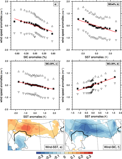
Figure 1. (a) Binned wind speed anomalies, as a function of binned sea ice concentration (SIC) anomalies (stars). (b)−(d) Binned monthly wind speed anomalies as a function of binned monthly sea surface temperature (SST) anomalies (stars) for open water, low ice concentration area (SIC < 20%) and high ice concentration area (SIC > 20%), respectively. Triangles are ± one standard deviation of wind speed anomalies within each bin. Red lines show regression. (e) Correlation between daily wind speed and SST. (f) Correlation between daily wind speed and SIC. Overlaid black contours in (e) and (f) show 20% SIC, with color-filled contours significant at the 95% level.
Download figure:
Standard image High-resolution image
Figure 2. (a) Long-term mean sea ice concentration (SIC) (%); (b) standard deviation for daily wind speed (m s−1); (c)−(d) composites of positive and negative wind speed anomalies (m s−1); (e)−(h) composites of sea surface temperature and surface air temperature anomalies (K) associated with positive and negative wind speed anomalies. Overlaid black contours in (c)−(d) are the corresponding composites of 20% SIC. P and N represent the strong and weak wind regime.
Download figure:
Standard image High-resolution image
Figure 3. Composite analysis results of (a) cloud fraction (%), (d) downward longwave radiation, (g) downward shortwave radiations, (j) sensible heat flux, and (m) latent heat flux in the strong wind speed regime. The unit of radiation and heat fluxes is (wm−2). (b), (e), (h), (k) and (n) are the same as those in (a), (d), (g), (j), and (m), but for the weak wind regime. (c), (f), (i), (l), and (o) show the differences between strong and weak regimes.
Download figure:
Standard image High-resolution image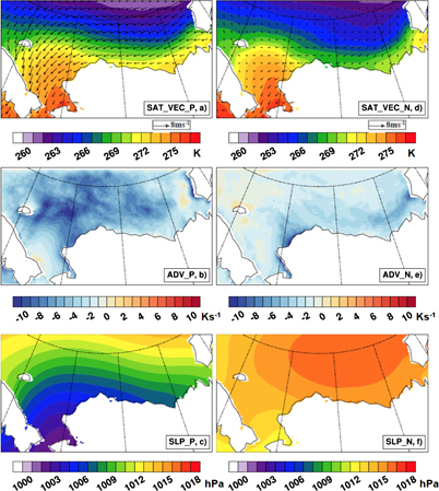
Figure 4. Composite results of (a) surface air temperature (K) and wind vector (m s−1, reference vector 8 m s−1), (b) surface thermal advection (K s−1 scaled by 10−5), and (c) sea level pressure (hPa) in the strong wind regime. (d)–(f) are the same as those in (a)−(c) but for the weak wind regimes.
Download figure:
Standard image High-resolution image
We further conducted binned scatter analysis to examine the relationship between surface wind speed and SST. Unlike in the tropical ocean or mid-latitude warm boundary current areas, the presence of sea ice may complicate wind–SST relationships. We therefore divided our analysis into three groups using SIC as an index from SIC equal to 0% (open water area, OW), greater than 0% but less than 20% (area with low ice concentration, LIC), and between 20%–100% (area with high ice concentration, HIC). This analysis by grouping SIC enables consideration of sea ice influence on the relationship between surface wind speed and SST. An overall inverse linear relationship occurs for OW and LIC areas (figures 1(b) and (c)), with the correlation coefficients of −0.93 and −0.98, respectively, at a 99% level of significance by t-test. Note that the correlation becomes smaller when SST is greater than zero for the OW area. However, in the HIC area, a positive correlation coefficient of 0.96 at a 99% level of significance was identified, though a relatively flat regression line is observed due to the smaller magnitudes of wind anomalies compared with those in LIC area (figure 1(d)). It is worthwhile to mention again that monthly data were used for the overall correlation analysis above. The analysis using daily data shows the highly consistent results, except that the undefined regression in figure 1(d) becomes relatively flat and the scatters of the wind anomalies from the regression lines become larger in all panels of figure 1 (figure S1 in supplementary material available at stacks.iop.org/ERL/13/034008/mmedia). These are due to higher frequency of variability of daily winds than sea ice and SST. In the following detailed analysis of spatial structures of wind–sea ice–SST relationship and associated physical processes, we will employ daily data. In addition, a close examination of figures 1(b)–(d) shows that SST anomalies in the HIC areas have smaller variations than in the OW and LIC areas. This is consistent with observations and reflects the impact of sea ice on SST variations (Rayner et al 2003). The relatively small correlation coefficient between surface wind and SST in the HIC areas may also suggest that ice weakens the coupling between ocean and atmosphere.
To better understand these correlations, we examined the spatial distributions of the correlation of wind speed with SST and SIC. As shown in figure 1(e), positive correlations between wind speed and SST occur in the central part of the study domain, i.e. the northern Chukchi Sea and the Beaufort Sea (or HIC area). This correlation changes to be negative in the southern part of the domain, i.e. the southern Chukchi Sea and the Bering Sea (or OW and LIC areas). By contrast, a negative correlation between wind speed and SIC appears in the HIC area (figure 1(f)). No significant correlation between wind speed and SIC is found in the OW and LIC areas, due either to no ice or less ice present there. Also note that, compared with the overall correlation analysis, the spatial distribution shows smaller correlation coefficients, which can be attributed to the large variability of surface winds (figures 1(a)–(d)).
The maximum correlations of wind speed with both SST and SIC occur in the northern Chukchi Sea (figures 1(e) and (f)). These spatial structures confirm the overall analysis shown in figures 1(a) and (d), and clearly show a division approximately by the 20% SIC contour between the areas with different wind–SST relationships. In addition, the areas with the positive wind speed–SST correlation and the negative wind speed–SIC correlation are the same as the areas with enhanced surface winds (Stegall and Zhang 2012). This comparison gives evidence that the increased surface wind speeds could be attributable to the decrease in sea ice and increase in SST. This is because the increase in prevailing easterly and northeasterly winds in the area (figure 4(a)) advects more multiyear ice westward and southwestward, which dynamically contribute to an increase or at least maintenance of sea ice coverage (e.g. Zhang et al 2003), rather than decrease in sea ice coverage as indicated by the negative wind speed–SIC correlation. Also, surface thermal contrast and resultant baroclinicity is the fundamental mechanism driving genesis of weather systems and influencing surface winds. Nevertheless, there are complex interactive or feedback processes involved in the surface wind–SIC–SST relationship. The analysis here is just one aspect of these two-way processes. The other aspect will be examined in the next section on how SIC and SST change in response to different surface wind regimes.
3.2. Physical interpretation of the statistically revealed wind–SST–sea ice relationships
To explore more complete physical processes responsible for shaping the wind–SST–SIC relationships, in particular how changed atmospheric conditions feed back to SST and SIC, we performed a composite analysis of the wind speed anomalies and associated parameters. The anomalies of wind speed and other parameters were calculated as departures from their temporal means at each grid cell of the study domain. The composite results were constructed by selecting positive and negative phases of domain-averaged wind speed anomalies, using a criterion of ± one standard deviation. The composite results represent strong and weak wind regimes. In the study area, climatological SIC ranges from 0% to more than 90% (figure 2(a)), with larger wind speed variation occurring over the LIC area and smaller variation over the HIC area. Standard deviations of wind speeds range from about 2.2−3.5 m s−1 (figure 2(b)).
3.2.1. Changes in SIC, SST and SAT associated with shift of surface wind regime
Figures 2(c) and (d) show the composite analysis results of wind speed anomalies in strong and weak wind regimes, where contours corresponding to 20% SIC are overlaid. A comparison of the 20% SIC indicates a poleward shift of the 20% SIC contour in the strong wind regime, reinforcing the correlation analysis results above that stronger winds coincide with less sea ice extent in the entire study domain. When examining the composite results of the SST and SAT anomalies (figures 2(e)–(h)), we found that positive (negative) SST and SAT anomalies generally occur over the northern Chukchi Sea and Beaufort Sea, i.e. the HIC area, in the strong (weak) wind regime, except that negative SAT anomalies only occur over the eastern Beaufort Sea in the weak wind regime. Opposite signs of SST and SAT anomalies appear over the southern Chukchi Sea and Bering Sea (i.e. the OW and LIC areas) and near the northern boundary of the study domain or the central Arctic between the strong and weak wind regimes. The relationship between wind and SIC/SST is the same as what was revealed in the correlation analysis above.
3.2.2. Changes in surface energy budgets associated with shift of surface wind regime
To understand the changes in SST/SAT associated with wind speed regimes or feedback of changed wind regime to SST/SAT as shown in the composite analysis above, we examined the composite results of primary heat energy sources (such as cloud-radiative forcing) in the strong and weak wind regimes. We also compared the differences between the two regimes. It is generally challenging for models to realistically simulate cloud and radiative variables. Wilson et al (2012) noted underestimate in Arctic clouds from a WRF model simulation, in which the NCAR/NCEP reanalysis was used as forcing. Walsh et al (2009) compared Arctic cloud and radiation in different reanalysis data sets and found that ERA-40 matches observations at Barrow better than other data sets, and the NCAR/NCEP reanalysis tends to underestimate Arctic cloud at Barrow. The CBHAR data set used here was developed using ERA-Interim to define model boundary conditions. It shows that cloud covers generally greater than 80% during our study period, which is in reasonably good agreement with observations at Barrow (Dong et al 2010).
The composite analysis indicates increases in cloudiness and downward longwave radiation, and decreases in downward shortwave radiation in the southern part of the domain when the wind shifts to a strong regime (figure 3). The maximum increase in cloudiness occurs along the Siberian coast and the northwestern coast of Alaska. The longwave radiation follows a similar spatial pattern. Due to the increase in cloudiness, the shortwave radiation decreases accordingly. Over the northern part of the domain, there exists decreased cloudiness and downward longwave radiation, and slightly increased downward shortwave radiation in the strong wind regime. The small changes in the downward shortwave radiation in this northern area between the two wind regimes are due to the weak downward shortwave radiation at such high latitudes. In addition, the net shortwave radiation change is also small in this HIC area because of the fully covered sea ice and high surface albedo. As a result, the increased (decreased) longwave radiation is the major radiative forcing for the warmed SST and SAT in the central part of the domain in the strong wind regime (figures 2(e) and (g)), and in the northern part of the domain in the weak wind regime (figures 2(f) and (h)).
When taking a close look at the southern Chukchi Sea and the Bering Strait in the southern part of the domain, the magnitude of the increased downward longwave radiation is smaller than that of the decreased downward shortwave radiation in the strong wind regime (figures 3(f) and (i)). This is because the clear-sky downward shortwave radiation is larger at these lower latitudes. The increased cloudiness causes a larger amount decrease in downward shortwave radiation. In addition, the relatively warm cloud consists of more water droplets than the cold cloud does in the north, which can effectively reduce downward shortwave radiation (not shown). As a result, the decreased downward shortwave radiation plays an important role in cooling SST and SAT in the strong wind regime (figures 2(e) and (g)).
Motivated by several studies showing the close physical connection between fluxes of sensible and latent heat and sea ice properties (e.g. Tetzlaff et al 2013), we also conducted composite analysis for surface sensible and latent heat fluxes (figures 3(j)–(o)). The composite analysis results here show that the largest positive sensible and latent heat fluxes occur in the southern Chukchi Sea and the Bering Strait along the Alaskan coast, i.e. the OW and LIC area, in both wind regimes. This suggests heat loss mainly from the open ocean to the atmosphere (upward flux is positive). But their magnitudes are more than three times smaller than the downward longwave radiation (figures 3(d) and (e)). In the northern part of the domain, there are negative sensible and latent heat fluxes. The positive fluxes increases and show larger values in the northern Bering Strait along the Alaskan coast in the strong wind regime than those in the weak wind regime, causing cold SST and SAT there. In the northern part, the sensible and latent heat fluxes just slightly cause a warming effect on the surface.
3.3.3. Changes in thermal advection associated with shift of surface wind regime
In addition to radiative forcing, thermal advection is also a major contributor to dynamically forming temperature distribution and changes, especially when strong winds and great temperature gradients are present. To understand this dynamic contribution, we conducted a composite analysis for SAT, wind vector, temperature advection, and SLP in the strong and weak wind regimes, respectively (figures 4(a)–(f)). A southward temperature gradient exists in both regimes. The easterly and northeasterly winds prevail in the strong wind regime and the northeasterly and southeasterly winds dominate in the weak wind regime. As expected from SAT and wind vector distributions in the strong wind regime, a strong cold thermal advection occurs over almost the entire study area, with the maximum value around the 20% SIC contour line. This cold advection from the HIC area to the OW and LIC areas obviously contributes to the cold SST and SAT anomalies in the southern Chukchi Sea and Bering Strait (figures 2(e) and (g)). For example, Vihma and Brümmer (2002) suggest that cold air flowing from ice to much warmer open water could produce a strong air–sea coupling and destabilize the atmosphere. So, associated with the strong cold advection mentioned above, clouds may form over the OW and LIC areas, and then accompanied precipitation and reduced downward shortwave radiation can further cool the SST and SAT.
To the north of the 20% SIC contour, there is also strong cold advection due to the large temperature gradient. However, this cold advection is obviously not strong enough to reverse the sign of the SST and SAT changes caused by the cloud-enhanced downward longwave radiation (figures 2(e) and (g) and figure 3(h)).
The thermal advection is weaker in the weak wind regime. Although cold advection still dominates the study area, warm advection is also found in the northern and western part of the domain (figure 4(e)). When SLPs are compared between the two wind regimes (figures 4(c) and (f)), it is clear that the strong winds in figure 4(a) result from a poleward shift of cyclone tracks and intensification of cyclone activities, while the weak winds in figure 4(d) are mainly associated with the Beaufort high. The intensified cyclone activities would be responsible for the increased cloud coverage in the southern part of the domain as identified above (figures 3(a) and (g)). The warm advection on the west side of the Beaufort high favors the formation of the Arctic stratus over the northern part of the domain (figures 3(d) and (g)) and positive SAT anomalies there (figure 2(h)).
In addition, winds may also impact surface thermal conditions via altering boundary layer structure. For example, strong winds can dynamically increase boundary layer mixing and weaken the inversion that often occurs over the HIC area (e.g. Lüpkes et al 2008). This may increase surface temperature as shown in the northern Chukchi Sea and the Beaufort Sea. However, investigation on these small-scale boundary layer mixing processes is out of the scope of this study and can be a topic of follow-up research.
Taken together, the negative correlation between winds and SST over the OW and LIC areas can be attributed to reduced shortwave radiation due to increased cloudiness, increased upward sensible and latent heat fluxes, and strong cold advection from sea ice towards the north when strong winds are present, or vice versa when weak winds occur. Over the northern Chukchi Sea and Beaufort Sea (i.e. the HIC area), the positive (negative) anomalies in cloud cover and associated downward longwave radiation associated with the strong (weak) wind regime predominantly result in a positive correlation between winds and SST.
4. Summary and discussion
The Arctic Ocean has changed dramatically, in which the largest decline of summer sea ice cover has occurred in the Pacific Arctic Ocean. These changes can naturally enhance and be a consequence of complex interactions between atmosphere, sea ice, and ocean. To reveal these interactions in the context of regional climate variability and change, we conducted a statistical analysis to examine overall relationships between surface winds, SST, and sea ice in the CBS, using the newly developed CBHAR data set. The result shows a significant negative correlation between the surface winds and SIC, further confirming that increased wind speeds are closely associated with the reduction in SIC (Stegall and Zhang 2012).
The relationships between surface winds and SST can be complicated by the presence of sea ice. Over the OW and LIC areas, the correlation is negative. But it changes to positive over the HIC area. These opposite correlations between surface winds and SST with different SICs further reveal a physically-driven spatial distribution of wind anomalies. It shows that stronger winds tend to occur along the ice edge where stronger baroclinicity is present. Thus, over the OW and LIC areas, wind speed increases toward the colder water and the HIC area. Over the HIC area, stronger winds occur towards the LIC area.
Beyond the baroclinicity mechanisms, the other related major atmospheric physical processes for shaping the wind–SST–sea ice relationships include radiative forcing, surface turbulent heat fluxes, and thermal advection, though sub-grid scale atmospheric and oceanic boundary layer mixing processes may have contributions too. In the strong wind regime, there are enlarged open water and poleward shifted and intensified cyclone activities, causing an increase in cloudiness and downward longwave radiation, and a decrease in downward shortwave radiation. Changes in sensible and latent heat fluxes and strong thermal advection also occur at the same time. In the northern Chukchi Sea and Beaufort Sea or the HIC area, the downward longwave radiation dominates over the downward shortwave radiation because the latter is weak at such high latitudes during the study period. High albedo associated with the sea ice cover further reduces the net shortwave radiation. As a result, the increased downward longwave radiation predominantly results in an increase in SST, leading to a positive correlation with surface winds.
In the southern Chukchi Sea and the Bering Strait or the OW and LIC areas, a relatively large decrease in downward shortwave radiation occurs alongside enhanced cyclone activities in the strong wind regime. This can be attributed to two reasons. First, the relatively warm cloud associated with storms in the south can include more water droplets, which effectively reduces cloudy-sky shortwave radiation, compared to cold cloud in the north. Second, associated with the strong cold advection from the north, there would be more low-level clouds forming over the warm ocean surface in the OW and LIC areas. As a result, the large decrease in downward shortwave radiation along with weak net shortwave radiation, increased upward sensible and latent heat fluxes, and strong cold advection contribute to the cooling of SST and the negative correlation between SST and winds. Qian et al (2012) found similar SST cooling under strong winds in the South China Sea. However, it is mainly due to an increase in evaporation/precipitation and a decrease in shortwave radiation.
Note that, as mentioned above, in addition to the atmospheric contributors, wind-driven ocean dynamics may also contribute to the relationship between wind and SST. Although the modeling system generating CBHAR does not explicitly includes ocean dynamics, it assimilated the observed SST. Accordingly, the CBHAR data implicitly includes the effects of ocean dynamics occurring in the real world. For the analysis here, strong winds can weaken ocean stratification and, in turn, mix the warmer surface water with the colder water underneath, causing a decrease in SST in the OW and LIC areas.
The weak wind regime occurs when the Beaufort high dominates the study area. The southeasterly winds over the west side of the Beaufort high bring warm air to the cold ice surface, favoring the formation of Arctic stratus cloud over the western and northern part of the domain. As a result, the enhanced downward longwave radiation and the resultant positive SAT anomalies occur. But no obvious SST anomalies appear due to the high SIC there. In the northern Chukchi Sea and the Beaufort Sea where SIC is greater than 20%, the small cloud-forced longwave radiation and weak downward shortwave radiation result in cooling of SSTs. The warmed SSTs over the LIC and OW areas result mainly from the enhanced downward shortwave radiation due to the lower latitudes and less cloud cover than in the north. Weak winds may also allow ocean stratification to persist in the LIC and OW areas, which favor a warming of ocean surface and contributes to the formation of the negative correlation between wind speed and SST.
The study here provides climatological relationships between wind–SST–ice, which serves as a reference to detect changes in air–ice–sea interactions. In particular, the study area is undergoing drastic changes in atmospheric circulation, including the recently manifested intensification of the Beaufort high (e.g. Zhang et al 2008, Moore 2012, Wu et al 2014). The impact of this change on the wind–SST relationship can be even more complicated, as ocean upwelling/downwelling forced by the circulation change can also impact the SST (e.g. Pickart et al 2011). Also, preconditioning of sea ice in preceding season would also influence air–ice–sea interactions in September and October. Persistence of the preconditioning and across-season influence of sea ice for certain decadal or multi-decadal time periods may lead to different wind–SIC–SST relationship. Meanwhile, effects of sea ice induced baroclinicity on surface wind may also be wind-direction-dependent as suggested by Chechin and Lüpkes (2017). In addition, we have analyzed how sea ice/SST induced baroclinicity influences surface winds and how thermodynamic processes associated with surface wind changes impact underlying sea ice and SST. However, linkage between these two aspects to form a feedback loop and persistence of this feedback with time remain unclear. So, to further understand the physics beyond the statistical relationships and the associated physical analysis here, and to fully untangle the complex interactive processes between atmosphere, sea ice, and ocean interactions, in particular in a rapidly changing Arctic climate, experiments using climate models, with complete atmosphere–ocean–sea ice feedback processes, would be required in follow-up studies.
Acknowledgments
This work was sponsored by BOEM/DoI (M06PC00018) and NSF (ARC-1023592). The CBHAR data set is archived at ARSC. Appreciation goes to Wei Tao for helping to finalize figure plots. We also thank the editor and anonymous reviewers for their insightful and constructive comments, which have helped improve the manuscript.