

Abstract
Climate extremes have the potential to cause extreme responses of terrestrial ecosystem functioning. However, it is neither straightforward to quantify and predict extreme ecosystem responses, nor to attribute these responses to specific climate drivers. Here, we construct a factorial experiment based on a large ensemble of process-oriented ecosystem model simulations driven by a regional climate model (12 500 model years in 1985–2010) in six European regions. Our aims are to (1) attribute changes in the intensity and frequency of simulated ecosystem productivity extremes (EPEs) to recent changes in climate extremes, CO2 concentration, and land use, and to (2) assess the effect of timing and seasonal interaction on the intensity of EPEs. Evaluating the ensemble simulations reveals that (1) recent trends in EPEs are seasonally contrasting: spring EPEs show consistent trends towards increased carbon uptake, while trends in summer EPEs are predominantly negative in net ecosystem productivity (i.e. higher net carbon release under drought and heat in summer) and close-to-neutral in gross productivity. While changes in climate and its extremes (mainly warming) and changes in CO2 increase spring productivity, changes in climate extremes decrease summer productivity neutralizing positive effects of CO2. Furthermore, we find that (2) drought or heat wave induced carbon losses in summer (i.e. negative EPEs) can be partly compensated by a higher uptake in the preceding spring in temperate regions. Conversely, however, carry-over effects from spring to summer that arise from depleted soil moisture exacerbate the carbon losses caused by climate extremes in summer, and are thus undoing spring compensatory effects. While the spring-compensation effect is increasing over time, the carry-over effect shows no trend between 1985–2010. The ensemble ecosystem model simulations provide a process-based interpretation and generalization for spring-summer interacting carbon cycle effects caused by climate extremes (i.e. compensatory and carry-over effects). In summary, the ensemble ecosystem modelling approach presented in this paper offers a novel route to scrutinize ecosystem responses to changing climate extremes in a probabilistic framework, and to pinpoint the underlying eco-physiological mechanisms.
Export citation and abstract BibTeX RIS

Original content from this work may be used under the terms of the Creative Commons Attribution 3.0 licence.
Any further distribution of this work must maintain attribution to the author(s) and the title of the work, journal citation and DOI.
1. Introduction
Climate variability and extremes are key features influencing terrestrial ecosystem functioning (Smith 2011, Reyer et al 2013, Baldocchi et al 2016). Climatic extremes directly propagate into the biosphere through various eco-physiological pathways, for instance affecting plant phenological events (Jentsch et al 2009, Ma et al 2015) or carbon cycling from regional to global scales (Knapp et al 2002, Reichstein et al 2013, Zscheischler et al 2014a, Frank et al 2015). Major climatic extreme events such as the European heat wave and drought in 2003 (Ciais et al 2005, Reichstein et al 2007), or droughts in North America (Schwalm et al 2012, Wolf et al 2016), Australia (Ma et al 2016) and the Amazon (Phillips et al 2009, Lewis et al 2011) consistently cause net carbon losses. However, because the number of directly observed large-scale extreme climate events and associated impacts on ecosystem productivity are rare, and because field experiments are often limited in extent and thus difficult to upscale to larger regions (Beier et al 2012), crucial uncertainties remain in our understanding of processes that control these phenomena.
Climatic extreme events are changing in magnitude and frequency (Alexander et al 2006, IPCC 2012), and these occur in addition to more gradual climatic changes in, e.g. seasonal variation (Stine et al 2009, Cassou and Cattiaux 2016) and climate trends. These changes, in tandem with non-linear feedbacks or lagged effects (Frank et al 2015), might impart decisive consequences for regional and global-scale carbon balances of terrestrial ecosystems (Reichstein et al 2013).
For example, the extreme summer drought 2012 in the contiguous United States caused losses in carbon uptake in summer (Wolf et al 2016) which were offset by warming-induced increases in spring carbon uptake, leading to a spring–summer compensation of the regional carbon balance (figure 1). Furthermore, Wolf et al (2016) hypothesized that earlier spring plant activity could have induced negative carry-over effects to summer productivity via soil-moisture deficits (figure 1), as suggested in Richardson et al (2010). However, as the evidence for seasonal compensation of extremes in Wolf et al (2016) is based on a single event only it remains uncertain whether such interacting effects can be expected generally for climate extremes in summer. Long time series allowing a comprehensive study of additional independent climatic extreme events in spring and/or summer would be required as such lagged effects in ecosystem productivity could have simply occurred by chance.
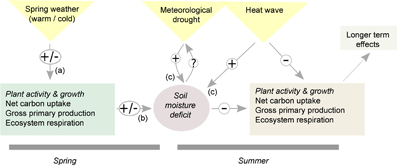
Figure 1 Conceptual illustration of spring-summer interacting carbon cycle effects due to climate extremes. In years affected by summer heat and drought (arrows (c)), warm spring conditions could potentially partly compensate for carbon losses in summer due to higher carbon uptake in spring (arrow (a), associated with (+)). Conversely, however, warm spring conditions might lead to earlier soil moisture depletion (arrow (b), associated with (+)) and thus a carry-over effect from spring to summer carbon cycling. Diagram modified from Sippel et al (2016b), CC BY 4.0.
Download figure:
Standard image High-resolution imageClimate extremes may cause immediate or delayed responses in ecosystems (Frank et al 2015), but not all climate extremes lead to an extreme ecosystem response (Smith 2011). Therefore, systematic quantification and attribution of contemporary trends in ecosystem productivity extremes, including potential interactions of events, is required. Respective analysis on observations is often hindered by small sample sizes. Alternatively, large ensembles of climate–ecosystem model simulations might complement a 'case study type' assessment of extremes in the observational record because they allow exploration of how climate variability and extreme events are related to extreme ecosystem responses (Ciais et al 2005, Schwalm et al 2012, Wolf et al 2016). For example, multi-thousand member ensembles of climate simulations were used to analyse and attribute extreme climate events, such as the Russian heat wave in 2010 (Otto et al 2012), or to investigate the role of climate extremes in causing, e.g. floods (Pall et al 2011, Schaller et al 2016) and heat-health related issues (Mitchell et al 2016). This approach is appropriate when analysing the impact of climatic extreme events on ecosystem functions.
This study investigates two main objectives: our first objective is to systematically assess changes in EPEs in spring and summer using climate–ecosystem model ensemble simulations, and to attribute seasonal changes in EPEs to changes in climate extremes, atmospheric CO2 and land-use change. Second, we focus on interactions between negative summer EPEs and the preceding spring conditions, and reinvestigate the outlined spring compensation and carry-over effects in years affected by negative summer EPEs on regional carbon cycling from a climate-ecosystem ensemble modeling perspective, and provide a model-based interpretation and generalization of these effects.
2. Data and methods
The methodological workflow of the study is as follows: we use a large ensemble of bias-corrected regional climate model simulations (section 2.1) to drive an ensemble of ecosystem model simulations (section 2.2) for six eco-physiologically different European regions. Factorial model simulations are set up (section 2.3) and used to disentangle climatic and non-climatic drivers of seasonal changes in EPEs, and to scrutinize respective spring-summer interacting carbon cycle effects (section 2.4).
2.1. Regional climate model simulations and physically consistent bias correction
The core ingredient to the present study is an ensemble of regional climate simulations over Europe that cover 26 years of transient climate change (1985–2010) and 800 ensemble members in each year (i.e. 20 000 members in total) based on perturbed initial conditions. Climate model simulations have been generated through distributed computing on citizen scientists' computers (www.climateprediction.net/weatherathome), using the global general circulation model HadAM3P (1.875° × 1.25°15 min resolution, 19 vertical levels) and a dynamically downscaled regional model version (HadRM3P, 0.44° × 0.44° × 5min resolution, Massey et al (2015)) in atmosphere-only mode. Hence, the model is driven by observed sea surface temperatures, sea ice fractions, the solar cycle, and the observed atmospheric composition (greenhouse gases, aerosols, ozone, see Massey et al (2015) for further details). The present experimental setup has been used to assess and attribute changes in climatic extreme events and its impacts in various sectors (Otto et al 2012, Sippel and Otto 2014, Schaller et al 2016, Mitchell et al 2016), because the large available sample size allows scrutiny of even small changes in the odds of climatic extreme events. The European summer climate in HadRM3P and other climate models is frequently too hot and dry (Massey et al 2015). To alleviate this issue, we apply a resampling-based bias correction that preserves the physical consistency in the ensemble simulations (for details see Sippel et al (2016a)): A Gaussian kernel fitted over 1985–2010 mean summer area-averaged temperatures in the ERA-Interim dataset (Dee et al 2011) in each of the six European regions (online supplementary table S1) is used as a constraint for resampling 500 ensemble members in each year. The resampling procedure improves the representation of summer climate in HadRM3P substantially, but reduces the available sample size of the ensemble and cannot account for all possible biases (Sippel et al 2016a).
2.2. Terrestrial ecosystem simulations: model description
The process-based Lund–Potsdam–Jena managed Land dynamic model (LPJmL, Version 3.5) simulates terrestrial vegetation dynamics (growth, competition and mortality), land–atmosphere fluxes of carbon (gross and net primary productivity, ecosystem respiration) and water (evaporation, transpiration, interception) in natural ecosystems (Sitch et al 2003) and under human land use (Bondeau et al 2007). Carbon allocation in LPJmL follows the fully coupled photosynthesis and water balance scheme of the BIOME3 model (Haxeltine and Prentice 1996), i.e. the photosynthetic light-use efficiency is subject to environmental controls via co-limiting light-limited enzyme regeneration and rubisco-limited enzyme-kinetic rates (Haxeltine and Prentice 1996). Respiration from plant compartments follows a modified Arrhenius relationship (Lloyd and Taylor 1994). Heterotrophic decomposition of litter and soil carbon pools depends additionally on soil moisture and follows first-order kinetics (Sitch et al 2003). LPJmL consists of 11 natural plant functional types and 13 crop functional types that differ in their bioclimatic limits and ecophysiological parameters. Here, we run LPJmL with an improved hydrology scheme (Gerten et al 2004, Schaphoff et al 2013), human land use (Bondeau et al 2007), agricultural water use (Rost et al 2008), and an improved phenology module (Forkel et al 2014). Phenology and photosynthesis-related parameters have been optimized against remote sensing observations resulting in an improved simulation of natural vegetation greenness dynamics (Forkel et al 2015). LPJmL ensemble simulations are performed at a monthly temporal and at 0.5° spatial resolution. The spinup procedure consists of 1200 years by randomly concatenating individual ensemble members (sampled from the first ten available years, 1986–1995) with transient CO2 concentration and land use.
2.2.1. Region selection
All ensemble simulations are conducted for six individual regions in Europe that broadly sample the spectrum of variability of vegetation productivity in Europe (online supplementary figure S1, available at stacks.iop.org/ERL/12/075006/mmedia), revealed from seasonal cycles in the satellite observed Fraction of Photosynthetically Active Radiation (FPAR) taken from the MODIS FPAR product (Myneni et al 2002). Spring (March–May) and summer (July–September) cover very different seasonality patterns in FPAR (figure 2). The LPJmL ensemble reproduces seasonal dynamics of vegetation phenology at the regional scale and the regional gradient in FPAR dynamics (figure 2).

Figure 2 (a) Illustration of seasonal cycles in vegetation phenology (indicated by the fraction of absorbed photosynthetically active radiation, FPAR) in satellite observations (MODIS) and in the ensemble of LPJmL model simulations (± 2σ range) in all six regions studied in this paper. (b) and (c) Identification of extremes in the response variable's distribution in the presence of trends in (b) spring and (c) summer: quantile regression of the 10th and 90th conditional percentile against time.
Download figure:
Standard image High-resolution image2.3. Factorial model simulations
The factorial set of climate–ecosystem model simulations (table 1) is based on a standard run ('All'), in which LPJmL is run with all drivers, including transient CO2 concentrations and human land-use (Fader et al 2010). Moreover, LPJmL is run separately for constant CO2 ('CONSTCO2'), constant land-use ('CONSTLU'), and both constant CO2 and land-use ('CONSTLUCO2'). In this factorial, ensemble-based setup the differences between these runs are used to disentangle and pinpoint climatic and non-climatic (CO2, land-use) drivers of contemporary changes in EPEs (sections 3.1 and 3.2). Lastly, to investigate carry-over effects from spring conditions to EPEs in summer (section 3.3), an additional LPJmL simulation driven by randomised spring climatic conditions ('SPRINGRAND') is conducted. This step consists of randomly concatenating members of the climate ensemble between summer and spring (on June 1st) within each year such that summer meteorology remains identical to the 'All' run, but spring conditions are different. Hence, the difference in summer carbon cycling between 'All' and 'SPRINGRAND' is driven by lagged effects from spring in the ecosystem model.
Table 1. Overview over factorial model simulationsa.
| Scenario name | CO2 | Land-use | Climate | Section |
|---|---|---|---|---|
| All | transient CO2 | transient land-use | transient climate | 3.1–3.3 |
| CONSTCO2 | constant CO2 b | transient land-use | transient climate | 3.1–3.2 |
| CONSTLU | transient CO2 | constant land-usec | transient climate | 3.1–3.2 |
| CONSTLUCO2 | constant CO2 b | constant land-usec | transient climate | 3.1–3.2 |
| SPRINGRAND | transient CO2 | transient land-use | transient climate, spring randomizationd | 3.3 |
aEach factorial simulation is conducted for 1986–2010 climate and propagated through the entire climate ensemble. bfixed to 345 ppm in 1985. cfixed to 1985 land-use values. dEnsemble members have been randomly concatenated on June 1st in each year ('random spring', but meteorological summer and autumn are identical to the other scenarios).
2.4. Analysis methodology
2.4.1. Selection of extreme events
All individual ensemble members are averaged to regional and seasonal means for further analysis. EPEs are sampled directly from the tail of the response variable distribution (Smith 2011), which is either gross primary productivity (GPP) or net ecosystem productivity (NEP) in the present study. Let xi,t,s,fac denote the response variable x (x ∈ {GPP, NEP}), an arbitrary ensemble member i, in year t, season s, and from any factorial run fac (region is not indexed separately to lighten the notation). Ensemble members in which the response variable exceeds or falls below a given threshold in the 'All' simulations are labelled as positive and negative EPEs ( and
and  , respectively). The index j runs only over ensemble members within in a given category (−extreme or +extreme). In section 3.1, an illustrative extreme value analysis is conducted by fitting a generalized Pareto distribution (GPD) to extremes in the response variable, where the GPD constitutes a suitable limit distribution for such peak-over-threshold selection of extreme values (Coles et al 2001). These statistical fits are derived from the 'All' simulations separately for the response variables's lower and upper tails (negative and positive EPEs) using a 5th and 95th quantile threshold to identify EPEs, and separately for each season and two decadal periods (1986–1995 and 2001–2010).
In sections 3.2 and 3.3, a quantile regression of the 10th (90th) conditional percentile against time in the 'All' simulation is performed (Cade and Noon, 2003) to identify EPEs relative to time-dependent thresholds, thus accounting for potential trends in the 25 year period. This yields a selection of 1250 EPEs (out of 12 500 members) for each response variable, region, and season (see figures 2(b) and (c) for an illustration).
2.4.2. Attribution to drivers of change
In section 3.1 (figure 3(b)–(e)), the effects of individual factors on changes in EPEs (CO2:  , land-use:
  , climate:
  , indicated here exemplarily only for negative extremes) between both periods and in season s are teased out by computing the difference between both time periods of the averaged individual effects from the factorial simulations (averages over any specific dimension (.) are denoted as
  ):
):
In section 3.2, the contribution of changes in CO2, land-use and climate to trends in EPEs are estimated individually for each tail, response variable, region and season. We assume linear trend slopes over the 25 year period and computed these in both tails separately (illustrated here for the negative tail,  ),
),
The contribution of trends in CO2  , land-use
  , and climate
  to changes in the response variable is determined from factorial model simulations, i.e.

Figure 3 (a) Seasonal cycle of NEP distribution as simulated by the LPJmL-ensemble for 1986–1995 and 2001–2010 in the France subregion. (b)–(e) Return time plots of seasonal NEP extremes (i.e. plotting the magnitude of an extreme event as a function of return time) in spring (b) and (d) and summer (c) and (e) for the upper (b) and (c) and lower (d) and (e) tail of the distribution for 1985–1995 and 2001–2010 (solid blue and orange lines, respectively, derived from fitting a generalized Pareto distribution (GPD) to threshold exceeding extremes in each tail, cf Coles et al (2001)). (b)–(e) Differences between the blue and orange lines indicate how the likelihood of extremes occurring has changed between the two compared decades. To illustrate the relative importance of individual drivers, we also plot the effects of changes in NEP that are driven individually by CO2, land-use, and climate from factorial model simulations depicted by the dashed lines, following equations (1)–(3). Full figure, including individual simulations is available in the supplementary data (figure S6).
Download figure:
Standard image High-resolution imageTo further examine climate-related drivers of change in ecosystem productivity, we analyse the individual contribution of trends in temperature, precipitation and radiation to  ). A simple statistical attribution framework is presented in the online supplementary data based on the 'CONSTLUCO2' scenario (supplementary section S1.2).
2.4.3. Spring–summer interacting carbon cycle effects due to climate extremes
In section 3.3, we identify all ensemble members that experience a negative EPE in summer (June–September, i.e.  ) using a time-dependent 10th percentile threshold. To detect spring compensation effects, we analyse the preceding spring conditions in the identified ensemble members in terms of ecosystem productivity anomalies that might potentially alleviate carbon losses in summer. Furthermore, the contribution of carry-over effects from spring to negative summer EPEs (e.g. via soil moisture depletion) is disentangled using factorial model simulations by analysing the difference between the 'All' and 'SPRINGRAND' simulations, i.e. with identical summer meteorology in both factorial simulations, but randomised spring meteorology. Hence, we compute spring–summer carry-over effects as the difference between the identified negative summer EPEs in both scenarios.
3. Results
In this section, we firstly illustrate in one region how large ensembles of climate–ecosystem model simulations can be used to study EPEs (section 3.1) and, secondly present a systematic assessment of spring and summer trends in EPEs and an attribution to drivers (section 3.2). Lastly, we investigate spring-summer interacting carbon cycle effects due to climate extremes (section 3.3).
3.1. An illustrative attribution analysis of ecosystem productivity extremes
The probability distributions of monthly GPP and NEP from the LPJmL ensemble in CEU-FRA for an earlier (1986–1995) and a more recent (2001–2010) period reveal an overall upward shift of GPP and NEP in spring but more nuanced changes in summer (figure 3(a) for NEP and online supplementary figure S5(a) for GPP). To investigate these changes in more detail, we apply an extreme value analysis to the tails of the probability distributions in both periods. Return time plots (figures 3(b)–(e)) for NEP and figures S5(b)–(e) for GPP) have been used widely in event attribution studies (National Academies of Sciences, Engineering and Medicine, 2016) to scrutinize the tails of a distribution by plotting the magnitude of an extreme event as a function of return time. Here, an event in the upper (lower) tail with an average return time of 20 years corresponds to a 95th (5th) percentile event when using annual data.
Differences between the blue and orange lines in figures 3(b)–(e) indicate how the likelihood of EPEs occurring has changed between the two compared decades for a given season and extreme type. In spring, terrestrial ecosystems exhibit an increase in GPP and NEP under extreme conditions in the upper and lower tail of the distribution in the more recent period (both tails shifted upward for any given return time, figures 3(b) and (d) and figures S5(b) and (d)). These increases are driven by a roughly equal positive contribution of climate and CO2 changes in the upper tail, and a larger contribution of climate change in the lower tail, in particular for GPP (figure S5(d)). Changes in the tails of the GPP distribution between both periods that are induced by individual drivers in the ecosystem model are largely additive, i.e. the average contribution of changes in CO2, land-use, and climate added to the statistical model for the 1986–1995 tail matches the statistical fit for the 2001–2010 tail (figures 3(b)–(e) and figure S5).
Changes in summer GPP are close to neutral, because the negative response to climate change is compensated by a positive contribution of CO2. NEP has significantly reduced (figures 3(c) and (e)), predominantly due to negative climate effects. For illustration, the European heat wave and drought of 2003 (figure 2(e), dashed horizontal line) results in a roughly 1-in-80 year event in the 1985–1995 decade but is already a 1-in-35 year event in the recent period. While the difference between the two decades used in this study is not comparable to a counterfactual climate simulation as utilised in other attribution studies (Mitchell et al 2016) it is reasonable to assume that the main difference in the climate simulations and thus NEP simulations comes from anthropogenic climate change.
Because ecosystem responses to climate extremes are often highly nonlinear and asymmetric depending on the type of extreme, changes in the likelihood of EPEs as discussed here are likely different from risk ratios based on meteorological variables alone (Stott et al 2004, Stott et al 2013). This study therefore exemplifies a simulation of the whole chain of events from meteorology to ecosystem responses in extreme event attribution (Stone and Allen 2005) and presents a framework for studying extreme ecosystem impacts.
3.2. Attribution of trends in ecosystem productivity extremes
Across all six European regions, trends towards increased gross productivity in spring for both positive and negative EPEs from 1986–2010 confirm a general upward shift in the GPP distribution (figure 4(a)) that is driven by both climate and CO2 changes. The pattern of an upward shift in spring is also found for NEP, but to a smaller extent that can be explained by a smaller sensitivity to recent changes in CO2 and climate (figure 4(b)). This is because recent climate change and CO2 fertilisation are not only enhancing primary productivity in spring but also ecosystem respiration, causing a smaller net response. Positive GPP trends are generally more than twice as large as NEP trends, i.e. less than half of the increased carbon uptake remains in the system after increased respiratory losses are accounted for, which is a consistent pattern for both positive and negative EPEs.
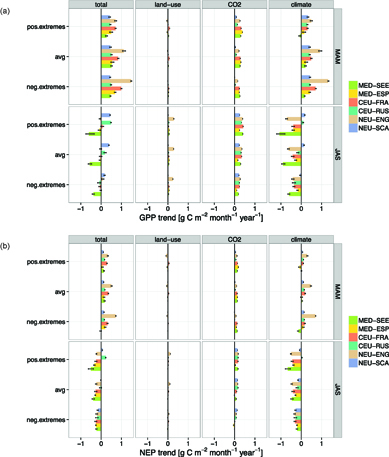
Figure 4 Factorial attribution of spring (MAM) and summer (JAS) trends in EPEs in six European regions to changes in land-use, CO2 and climate, for (a) GPP, and (b) NEP, as simulated by LPJmL.
Download figure:
Standard image High-resolution imageIn summer, the response of ecosystem productivity to recent climate change reverses (with few exceptions), but remains positive for CO2 changes: Hence, predominantly negative ecosystem productivity responses to recent climate change are balanced by a positive response to CO2 change, causing a mix of slightly increased (two regions), close-to-neutral (three regions) and reduced (one region) gross carbon uptake. Summer increases are confined to energy-limited regions in northern Europe (NEU-SCA and CEU-RUS) and more pronounced for the upper tail of GPP because the response of positive EPEs to recent climate change is marginally positive (in contrast to the other regions, figure 4(a)). Similar to spring, summer NEP trends are generally smaller in magnitude than GPP trends, and almost exclusively negative. The observed negative trends in summer ecosystem productivity and EPEs are most pronounced in water-limited regions in southern Europe (MED-SEE, MED-ESP, CEU-FRA) with relatively similar trend slopes in the upper and lower tail. The energy-limited regions in northern Europe experience reduced summer productivity under negative EPEs, but small increases in NEP under positive EPEs due to slightly different climate responses in the upper and lower tail (figure 4(b)).
Overall, LPJmL ensemble simulations reveal that seasonally contrasting responses of EPEs to changing climate conditions will be a crucial factor in determining regional-scale carbon balances in the near future. Further analyzing climate-induced trends in spring and summer ecosystem productivity ( and
and  ) in the online supplementary data (sections S1.2 and S2.2) reveals that climate-induced positive productivity trends are mostly driven by warming temperatures in spring (GPP: figure S7, NEP: figure S8), whereas the ecosystem response to summer warming is negative for NEP and GPP across Europe (except GPP in NEU-SCA).
3.3. Elucidating spring–summer interacting carbon cycle effects due to climate extremes
In 2012, the contiguous United States experienced a very warm spring followed by an extreme summer drought. Wolf et al (2016) hypothesized that warmer spring conditions and elevated spring plant activity might have induced soil moisture deficits, thereby exacerbating the impacts of summer drought (figure 1). Here, we analyse lagged effects in all ensemble members that experience extreme reductions in summer productivity7 (negative EPEs). Specifically, we investigate
- whether productivity losses induced by summer droughts are (increasingly) compensated by warmer spring conditions ('spring compensation', conceptual link (a) in figure 1), and
- whether spring–summer 'carry over effects' via soil moisture depletion further exacerbate negative EPEs in summer (conceptual link (b) in figure 1)?
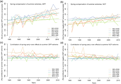
The conditional selection of summer extremes over NEU-ENG (figure 5(a)) shows that negative summer extremes can be preceded by various ecosystem productivity conditions in spring (figure 5(a)), i.e. there is no obvious deterministic link. However, there is indeed a probabilistic link between carbon cycling under summer extremes and the preceding spring productivity conditions, as four out of five European regions show, on average, increased spring GPP that compensates to a small extent for summer reductions (2.7%–19.0% average compensation, table 2), but smaller effects are observed for NEP (−4.3% to +7.8%). The MED-SEE region is an exception where summer extremes co-occur with on average reduced spring productivity (−4.6% in GPP and −10.4% in NEP of the summer anomaly are in addition lost in spring). Moreover, elevated ecosystem productivity in spring (GPP, and less so NEP) is increasingly compensating reductions in summer productivity in all European regions over the past 25 years (figure 6), albeit average spring compensation of negative EPEs in summer can only account for a fraction of the summer anomaly. These trends might be a consequence of seasonally contrasting trend slopes (sections 3.1 and 3.2).

Figure 5 Spring–summer interacting carbon cycle effects due to climate extremes illustrated in one region (NEU-ENG). (a) Association of spring anomalies with summer (June–September) anomalies in individual ensemble members. (b) Differences in soil water content explain spring-summer carry-over effects in the carbon cycle. The average spring compensation and contribution of carry-over effects to negative EPEs in summer are indicated by a horizontal red arrow in (a) and vertical red arrow in (b), respectively. Marginal distributions are plotted at the edge of each plot as individual ticks for all ensemble members (gray) and negative summer extremes (red).
Download figure:
Standard image High-resolution imageTable 2. Spring compensation of summer extremes in GPP and contribution of dynamical effects.
| Region | Variable | Summer extreme | Spring compensation | Carry-over effect | ||||
|---|---|---|---|---|---|---|---|---|
| Mean (gC m−2 month−1) | Mean (gC m−2 month−1) | Meana (% of summer anomaly) | Trenda,b(% year−1) | Mean (gC m−2 month−1) | Mean (% of summer anomaly) | Trendb (% year−1) | ||
| NEU-SCA | GPP | −24.0 | 5.6 | 19.0 | 1.7⁎ | −2.8 | 11.5 | −0.1 |
| NEU-ENG | GPP | −36.1 | 6.2 | 13.2 | 2.1⁎ | −8.5 | 23.5 | −0.4⁎ |
| CEU-RUS | GPP | −38.2 | 5.7 | 11.3 | 1.0⁎ | −3.3 | 8.3 | 0.0 |
| CEU-FRA | GPP | −33.7 | 1.0 | 2.7 | 1.7⁎ | −4.8 | 14.4 | −0.1 |
| MED-SEE | GPP | −34.3 | −2.1 | −4.6 | 0.7⁎ | −3.1 | 8.6 | 0.1 |
| NEU-SCA | NEP | −19.5 | 2.0 | 7.8 | 0.3⁎ | −1.9 | 9.1 | 0.2⁎ |
| NEU-ENG | NEP | −27.2 | 1.5 | 3.8 | 1.2⁎ | −5.1 | 19.1 | −0.8⁎ |
| CEU-RUS | NEP | −32.2 | 1.4 | 3.3 | 0.5⁎ | −2.0 | 6.0 | 0.0 |
| CEU-FRA | NEP | −27.3 | −1.6 | −4.3 | 1.0⁎ | −2.9 | 11.1 | −0.4⁎ |
| MED-SEE | NEP | −24.9 | −3.5 | −10.4 | 0.4⁎ | −2.1 | 8.7 | −0.4⁎ |
aThe sign is reversed for the computation of spring compensation relative to the summer anomaly for ease of understanding. bSignificance of the trend slopes at the 5% confidence level is indicated by an asterisk (⁎).
Figure 6 Trends and interannual variability in spring-summer interacting carbon cycle effects due to climate extremes in summer. (a), (c) Spring compensation of negative summer EPEs in (a) GPP, and (b) NEP. (b), (d) Contribution of spring-summer carry-over effect to negative summer EPEs in (b) GPP, and (b) NEP.
Download figure:
Standard image High-resolution image
3.3.1. Is there a causal link between spring carbon cycling and summer extremes?
Carry-over effects from spring to summer contribute on average 8.3%–23.5% for GPP (6.0%–19.1% for NEP) to the magnitude of extreme productivity reductions in summer (negative EPEs, see figure 5(b) for an illustration). This carry-over contribution is revealed by analysing differences in summer EPEs in the 'All' and 'SPRINGRAND' simulations (table 1), where summer meteorology is identical but spring conditions randomized in the latter simulation. Hence, summer ecosystem productivity extremes would be less severe if they would have been preceded by random spring conditions. The carry-over effects simulated by LPJmL are due to soil moisture depletion, because differences in soil moisture content explain a large fraction of the magnitude of carry-over effects across all regions (online supplementary table S2, figure 5(b) for NEU-ENG). These carry-over effects have been largely stable over the last 25 years (figure 6).
In summary, the analyses presented here provide an independent process model explanation and generalization of the observed seasonal compensation mechanism (Wolf et al 2016). However, we find that the average spring compensation of summer extremes is relatively small for GPP, almost neutral for NEP, and even negative (spring amplification of summer extreme) in MED-SEE for both GPP and NEP. Conversely, carry-over effects from spring to summer extremes via soil moisture play an important role in shaping simulated EPEs and exacerbate carbon cycle impacts on average. Hence, a substantial contribution of compensation effects (as observed for the 2012 US event, (Wolf et al 2016)) cannot generally be expected at present in Europe, and the role of these effects remains to be quantified on larger spatial scales, including uncertain long term legacy effects of climate extremes (Anderegg et al 2015). Furthermore, positive compensation trends as found for recent years (figure 6) cannot continue indefinitely, simply because there are natural limits to shifts in ecosystem phenology (Körner and Basler, 2010) and plant physiological responses to warming (Norby and Luo 2004).
4. Discussion
The results of our study provide evidence that EPEs in European ecosystems show a seasonally contrasting response to changes in climate when investigated using a large ensemble of ecosystem model simulations. Spring climatic changes tend to shift the GPP and NEP distribution upwards (including extremes in the upper and lower tails), whereas climatic changes in summer, most notably warming, lead to approximately neutral (GPP) or even negative trends (NEP), i.e. intensified carbon losses under climate extremes. Further, summer carbon losses as a result of climate extremes are partly compensated by a higher uptake in the preceding spring in temperate regions, but these spring compensatory effects are largely undone through a negative carry-over effect from spring to summer via depleted soil moisture, which further exacerbates summer carbon losses. Hence, our analyses provide a model generalization and interpretation of seasonal compensation and carry-over effects of carbon-cycle extremes.
However, the results of the present analysis might be confined by the fact that the underlying climate ensemble is based on just one regional climate model and uncertainties related to simulated trends, changes in (individual) climate variables, potential feedback mechanisms, and the applied bias correction remain (Massey et al 2015, Sippel et al 2016a).
Ecosystem models are derived from well-established theory of plant-atmosphere carbon exchange (Bonan 2015), and are widely analysed in the context of climate extremes (Ciais et al 2005, Reichstein et al 2007, Zscheischler et al 2014a). Nonetheless, the results presented here can still be influenced by scale mismatches, where models scale carbon assimilation from leaf to the ecosystem scale (Rogers et al 2017), or ecophysiological processes are simulated without considering a diurnal cycle and averaged over 0.5° grid cell size.
Moreover, a possible caveat of the present study is that ecosystem and carbon cycle models tend to overestimate the response of terrestrial carbon cycling to drought conditions if compared to observations-based datasets (Huang et al 2016). LPJmL and related earlier versions have been shown to overestimate the sensitivity of ecosystem productivity to precipitation deficits in central European regions as compared to tree ring data (Babst et al 2013), albeit qualitative responses are largely captured (Rammig et al 2015). Temperature extremes that are not associated with precipitation deficits are not affected (Rammig et al 2015). On the continental scale in Europe, extremes in LPJmL simulated GPP respond more sensitively to climate extremes than data-driven products, but in a qualitatively consistent way considering for example the ratio between positive and negative GPP extremes in Europe (Zscheischler et al 2014b). In this context, comparing the upper and lower tail of simulated ecosystem productivity in this study (figure 3(c) vs. figure 3(e)) reveals that extreme carbon losses in the lower tail are larger in magnitude than gains due to positive EPEs for a given return period (slopes in the return time plots in the lower tail exceed those in the upper tail for both GPP and NEP). This asymmetry in EPEs is consistent with analyses at the continental and global scale in observations-based products (Zscheischler et al 2014b). Van Oijen et al (2014) compares ecosystem productivity simulations and the vulnerability to precipitation deficits to satellite observations of vegetation greenness and finds that LPJmL (and other vegetation meodels) largely reproduce spatial patterns across Europe. Furthermore, the LPJmL version used in the present study incorporates a phenology scheme that improves phenological dynamics and variability of FPAR (Forkel et al 2015), and thus might overcome one of the previously identified key weaknesses of earlier LPJmL versions (Mahecha et al 2010).
Nonetheless, the analysis and attribution of simulated EPEs ignores a number of ecosystem processes and potential feedbacks between these, as these are missing in the LPJmL ecosystem model (e.g. wind disturbance, pests, nitrogen and phosphorous limitations) and generally many ecosystem processes and feedbacks during climatic extreme events are still unknown or uncertain (Reichstein et al 2013, Frank et al 2015). Hence, model improvements can only be conducted in synthesis with improving our process understanding of climatic extreme events. Therefore, dedicated ecosystem manipulation experiments (Knapp et al 2002, Jentsch et al 2007, Beier et al 2012) will be crucial to evaluate and scrutinize model predictions.
Despite these caveats, we argue that the analyses and tools presented here are useful to investigate specific hypotheses related to extremes in terrestrial ecosystems. Our approach allows a physically consistent probabilistic assessment of extremes in ecosystem productivity. Because the outlined probabilities and return times of EPEs are based on one ecosystem model, they should not be taken at face value, but rather be regarded as an approach to scrutinize model sensitivities and attribute drivers behind contemporary changes in ecosystem risk on decadal time scales.
An application of the analysis metrics developed for this study to other process-oriented ecosystem models or data-driven approaches (Tramontana et al 2016) could be one way to sample respective ecosystem model uncertainties, and to further scrutinise various hypotheses about interacting and contrasting contemporary changes in the frequency and intensity of ecosystem productivity extremes. Thereby, our suggested ensemble analyses might complement state-of-the-art ecosystem risk assessments (Van Oijen et al 2014, Rolinski et al 2015) and possibly guide ecosystem manipulation experiments towards pinpointing the most relevant and uncertain drivers of contemporary change in ecosystem extremes.
5. Conclusion
In this paper, we illustrate large ensemble simulations of ecosystem productivity as a useful tool to explore variability and change in EPEs from a probabilistic perspective. The approach allows to identify the drivers of changes in EPEs using attribution-type analyses (Stott et al 2013) and to analyse interacting carbon cycle effects caused by climate extremes (i.e. compensatory and carry-over effects). We find contrasting trends in spring vs. summer carbon cycle extremes in six eco-physiologically different European regions. A recent upward shift in the distribution of spring ecosystem productivity (including extremes) can be attributed to recent climate warming and CO2 increases, whereas in summer, ecosystem extremes are intensifying for NEP (i.e. more carbon lost to the atmosphere under drought and heat conditions) and roughly stable for GPP, despite a positive response to increasing CO2. Despite these overarching trends, regional differences are emerging, in that water-limited regions in southern Europe show smaller trends in spring, hence benefitting to a smaller degree from warming, while negative trends in summer net ecosystem productivity and its extremes are least pronounced in temperature-limited northern regions.
Furthermore, spring GPP increasingly compensates negative EPEs in summer GPP in four out of five European regions. However, this compensation occurs only partly, on average in the range of 2.7%–19.0% of the summer anomaly, but depends on the definition of extremes (figure 5). Spring compensation effects and trends are smaller but mostly positive for NEP. Conversely, spring–summer carry-over effects exacerbate carbon cycle losses under summer extremes (contribution of 8%–23% in GPP and 6%–19% in NEP to summer anomaly), thereby counterbalancing and undoing positive compensation-related effects. Therefore, we expect that climate extremes increasing in frequency and intensity (IPCC 2012) might further exacerbate legacy effects of ecosystem extremes in the long term beyond the actual events (Anderegg et al 2015).
Acknowledgments
We thank Nuno Carvalhais, Kazuhito Ichii, Martin Jung, Sonia I. Seneviratne, and Sebastian Wolf for helpful comments and discussions. We would like to thank our colleagues at the Oxford eResearch Centre for their technical expertise, the Met Office Hadley Centre PRECIS team for their technical and scientific support for the development and application of weather@home and all volunteers who have donated their computing time to climateprediction.net. ERA-Interim data provided courtesy ECMWF. This research has received funding from the European Commission Horizon 2020 BACI Project (Towards a Biosphere Atmosphere Change Index, grant No. 640176). SS is grateful to the German National Academic Foundation (Studienstiftung des Deutschen Volkes) for support and the International Max Planck Research School for Global Biogeochemical Cycles (IMPRS-gBGC) for training.
Footnotes
- 7
The subregion over Spain is excluded from the analysis because seasonality in ecosystem productivity differs strongly from other European regions, see figure 2.