
Abstract
Recent advances in remote sensing and ecological modeling warrant a timely and robust investigation of the ecological variables that underlie large-scale patterns of breeding bird species richness, particularly in the context of intensifying land use and climate change. Our objective was to address this need using an array of bioclimatic and remotely sensed data sets representing vegetation properties and structure, and other aspects of the physical environment. We first build models of bird species richness across breeding bird survey (BBS) routes, and then spatially predict richness across the coterminous US at moderately high spatial resolution (1 km). Predictor variables were derived from various sources and maps of species richness were generated for four groups (guilds) of birds with different breeding habitat affiliation (forest, grassland, open woodland, scrub/shrub), as well as all guilds combined. Predictions of forest bird distributions were strong (R2 = 0.85), followed by grassland (0.76), scrub/shrub (0.63) and open woodland (0.60) species. Vegetation properties were generally the strongest determinants of species richness, whereas bioclimatic and lidar-derived vertical structure metrics were of variable importance and dependent upon the guild type. Environmental variables (climate and the physical environment) were also frequently selected predictors, but canopy structure variables were not as important as expected based on more local to regional scale studies. Relatively sparse sampling of canopy structure metrics from the satellite lidar sensor may have reduced their importance relative to other predictor variables across the study domain. We discuss these results in the context of the ecological drivers of species richness patterns, the spatial scale of bird diversity analyses, and the potential of next generation space-borne lidar systems relevant to vegetation and ecosystem studies. This study strengthens current understanding of bird species–climate–vegetation relationships, which could be further advanced with improved canopy structure information across spatial scales.
Export citation and abstract BibTeX RIS

Content from this work may be used under the terms of the Creative Commons Attribution 3.0 licence. Any further distribution of this work must maintain attribution to the author(s) and the title of the work, journal citation and DOI.
1. Introduction
Ecologists have long sought to explain the distribution patterns of species diversity, which is an increasingly important research goal as climate change is expected to alter these patterns considerably (e.g. Parmesan 2006, Bellard et al 2012). Animal species richness and abundance distribution patterns have often been explained in terms of environmental variables, including climate and vegetation properties (e.g. Kerr 2001, Ricklefs 2004, Ceballos and Ehrlich 2006, Mittelbach 2010). Past work hypothesized animal species richness is more strongly related to climate and energy (e.g. productivity) at large spatial scales but more closely related to habitat diversity at regional to local scales (Blackburn and Gaston 1996, Currie et al 1999, Deppe and Rotenberry 2008, Kerr 2001, Kerr and Packer 1997, Mittelbach et al 2001). The relative importance of these environmental variables for predicting bird species richness has been explored at various scales (e.g. Cueto and Casenave 1999, Seoane et al 2004, Coops et al 2009, Hinsley et al 2009, Hansen et al 2011, Bar-Massada et al 2012, Fitterer et al 2012), but is still not well defined across scales. This is partly because measurements of vertical habitat heterogeneity and canopy structure (i.e. the horizontal and vertical distribution of canopy elements) have not been widely or consistently available across a range of locations, despite having long been recognized as important determinants of microclimates and microhabitats, and consequently the abundance and distribution of species (MacArthur and MacArthur 1961, Whittaker et al 2001).
Light detection and ranging (lidar) is advancing field-based understanding of these ecological interactions by providing novel information on spatial and vertical canopy structure and the impact of this structure on habitat diversity and quality (Bergen et al 2009, Lefsky et al 2002, Turner et al 2003, Vierling et al 2008). There is now a rapidly growing number of studies utilizing airborne lidar for biodiversity research, and many studies have found moderate to strong relationships between remotely sensed vegetation canopy structure, habitat quality, species richness and abundance, and habitat use (Bradbury et al 2005, Clawges et al 2008, Goetz et al 2010, 2007, Hill et al 2004, Lesak et al 2011, Seavy et al 2009, Swatantran et al 2012). However, these studies have been limited because airborne lidar data is generally not available over large areas. Consequently it has been difficult to test hypotheses relating the impact of variations in canopy structure to bird species richness patterns over large scales in a systematic fashion. A unique global vegetation canopy structure data set was acquired from space by GLAS (GeoScience Laser Altimetry System) onboard ICESat (the Ice, Cloud, and Land Elevation Satellite) from 2003 to 2009 (Schutz et al 2005). The GLAS data set provides the first opportunity to explore the importance of structure relative to other vegetation properties over large spatial extents and across broad gradients in climate and other environmental factors.
Here we investigate the patterns of breeding bird species richness across the coterminous United States and southern Canada, a domain established by the existence of well-documented bird observation data sets provided by the North American Breeding Bird Survey (BBS) (Pardieck and Sauer 2007, Ralph et al 1995) (figure 1). We predict species richness using models that incorporate a range of environmental and vegetation variables, and assess the relative importance of different influences on bird richness patterns across the study domain. Important aspects of this work include; (i) derivation and use of a range of satellite remote sensing variables, including vegetation canopy structure metrics, (ii) application of climate data that capture extremes and variability as well as mean conditions, (iii) application of advanced machine learning methods (ensembles of regression trees) for data mining and predictive model development within buffer zones surrounding BBS routes, (iv) robust model results and cross validation, (v) production of continuous, relatively high resolution (1 km) maps of species richness for various bird habitat guilds. Whereas some of these topics have been explored in past biodiversity research (see above), few have incorporated all of these elements or considered the relative importance of factors driving species richness patterns consistently across large spatial extents and a diversity of habitat types.
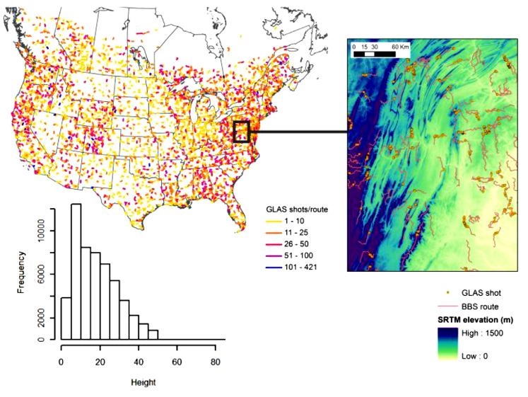
Figure 1. Distribution of BBS routes throughout North America and the number of GLAS lidar shots within 200 m of each route (upper left). The inset details the locations of the GLAS shots (right) and the histogram shows their height (m) distribution (lower left).
Download figure:
Standard image High-resolution image2. Methods
We assessed 47 bioclimatic and vegetation predictor variables of bird species richness (our response variable) for different guild types and in aggregate. We explored statistical associations and the strength of Pearson correlation coefficients for each predictor variable with species richness. We also used Random Forests, a regression tree method that calculates the average of an ensemble of individual trees using bootstrapped sampling (Cutler et al 2007), to predict species richness. When compared against other species distribution models, Random Forests has consistently performed well (e.g. Lawler et al 2006, Cutler et al 2007). One advantage of the random forest method is that provides us a mechanism for interpreting how important each of the predictor variables are (i.e. their explanatory power) and how results change as predictor variables are changed (so-called partial dependence plots, described below).
2.1. Bird species richness variables
2.1.1. Breeding bird survey
We used data acquired, compiled and distributed by the BBS, which was launched in 1966 to characterize avian population trends along survey routes through time (Pardieck and Sauer 2007, Ralph et al 1995). Bird counts are conducted annually at the peak of the nesting season along ∼4100 randomly selected routes throughout the United States and Canada (www.pwrc.usgs.gov/bbs). Along each 40 km route, a trained observer conducts stops about every kilometer and records all birds heard or seen within a 3-min period. The BBS data are publically available (ftp://ftpext.usgs.gov/pub/er/md/laurel/BBS/DataFiles).
We note that a potential source of error in using BBS data to derive species richness is the lack of complete detectability of all species that occur along a route (Boulinier et al 1998). Nichols et al (1998) developed a series of estimators based on capture–recapture theory to account for incomplete detection among species. The approach, however, requires assumptions that may not be met on BBS routes (e.g. closed populations, equal detection probabilities along routes) and other studies have found results of continental scale bird richness had similar results with and without the correction (Hansen et al 2011, Phillips et al 2010). Thus, we elected not to apply detectability corrections here.
We used the yearly summary data for each route for the years 2004–2006 (inclusive), which most closely matched the timeframe of the other data sets (predictor variables) with which we were working. Only routes and species with all three years of data were used. Bird species richness was thus derived for each of more than 3000 BBS routes in the coterminous US with a full suite of predictor variable data. We summed bird observations across all stops along each route for all three years. The number of unique species recorded totaled 668. We then used these species richness estimates as the response variable in the model development and analyses that follow.
2.1.2. Bird habitat guilds
We categorized and independently analyzed richness of bird species within breeding habitat groups (guilds) using the system developed by Peterjohn and Sauer (1993). We focus on four habitat guilds (forest, open woodland, grassland and scrub) comprising 69% of the total number of observed individuals and 61% of the total number of species (table 1). These guilds were also most broadly geographically distributed and most relevant in terms of terrestrial vegetation habitat, allowing analyses of the greatest number of bird species across a broad range of vegetated habitat types and ensuring a sufficient number of observations for statistically robust analyses.
Table 1. Bird breeding habitat guilds, with the number of bird species, their abundance, and the number of BBS routes with data for that specific guild. The top four guilds were selected for analysis.
| Habitat guild | Routes | Species |
Individuals |
|---|---|---|---|
| Forest | 1239 | 123/20 | 969 401 |
| Open woodland | 1308 | 105/20 | 2 036 529 |
| Grassland | 1285 | 60/6 | 941 448 |
| Scrub | 1286 | 45/7 | 313 590 |
| Deserts | 68 | 8 | 8 034 |
| Town | 1223 | 12 | 760 215 |
| Shore-line | 320 | 45 | 45 030 |
| River/stream | 197 | 3 | 1 457 |
| Lake/pond | 1231 | 55 | 403 344 |
| Ocean | 17 | 32 | 5 606 |
| Marsh | 1203 | 59 | 665 849 |
| Top 4 guilds | — | 333 | 4 260 968 |
| Other guilds | — | 214 | 1 889 535 |
| Top 4% of total | — | 61% | 69% |
aThe number of species considered in this study. bThe number of species from Matthews et al (2011) considered in this study.
2.1.3. Predictor variables
The predictor variables were selected to represent a spectrum of habitat characteristics that could potentially influence the richness of bird species in any particular area. We separated these into three broad categories: physical environment (20 climate and topography variables), vegetation properties (15 variables), and canopy structure (9 variables). We considered structure metrics separately because they have been the subject of much interest in the context of three-dimensional habitat heterogeneity, as opposed to the two (horizontal) dimensions represented by the other variables, but also because they were derived from a satellite sensor that provides samples as opposed to wall-to-wall coverages (images). These variables are listed in table 2 and are described in more detail below. Because our focus was on physical environment and vegetation, we did not consider detailed predictors of human impact such as housing density, roads or impervious cover. These factors have been well examined by other studies and been shown to sometimes have strong local effects on bird communities (Beaudry et al 2013, Pidgeon et al 2007, Suarez-Rubio et al 2013).
Table 2. Naming convention and brief description of the predictor variables and their source. Variables are organized according under broad categories including canopy structure, (other) vegetation properties, and physical environment. Elevation and all of the structure variables are in units of height (m) with the exception of COMP, VDR, Npeaks (unitless), and AreaBE, AreaCD (m2). Units of temperature (°C) and precipitation (mm) are used. VCF, Life Form, and Tree Leaf metrics are proportional (%). Biomass is (Mg ha−1) and NPP (gC m−2 yr−1).
| Variable name | Variable description | Source | |
|---|---|---|---|
| Canopy structure | CH | Canopy height | GLAS lidar |
| HOME | Median energy of the lidar waveform | GLAS lidar | |
| COMP | Waveform complexity | GLAS lidar | |
| Npeaks | Number of peaks in the waveform | GLAS lidar | |
| AmpMax | Maximum amplitude of the waveform | GLAS lidar | |
| AreaBE | Area under the waveform | GLAS lidar | |
| CD | Height (depth) of the canopy layer | GLAS lidar | |
| AreaCD | Energy under the canopy layer | GLAS lidar | |
| VDR | Canopy vertical distribution ratio | GLAS lidar | |
| Vegetation properties | NPP | Net primary productivity | MODIS-17A3 |
| EVIarea | Integrated EVI during the growing season | MODIS-12Q2 | |
| VCF | Vegetation continuous fields (canopy cover) | MODIS-44B | |
| Biomass | Biomass density | CONUS | |
| LFcrop | Life form: crops | SYNMAP | |
| LFgrass | Life form: grass | SYNMAP | |
| LFshrub | Life form: shrub | SYNMAP | |
| LFtree | Life form: trees | SYNMAP | |
| LFurban | Life form: urban | SYNMAP | |
| LLmixed | Tree leaf longevity: mixed | SYNMAP | |
| LLeverg | Tree leaf longevity: evergreen | SYNMAP | |
| LLdecid | Tree leaf longevity: deciduous | SYNMAP | |
| LTbroad | Tree leaf type: broad | SYNMAP | |
| LTmixed | Tree leaf type: mixed | SYNMAP | |
| LTneedle | Tree leaf type: needle | SYNMAP | |
| Physical environment | SRTM | Elevation (meters) | SRTM |
| bio1 | Annual mean temperature | WorldClim | |
| bio2 | Mean diurnal range (mean of monthly values) | WorldClim | |
| bio3 | Isothermality | WorldClim | |
| bio4 | Temperature seasonality | WorldClim | |
| bio5 | Max temperature of warmest month | WorldClim | |
| bio6 | Min temperature of coldest month | WorldClim | |
| bio7 | Temperature annual range | WorldClim | |
| bio8 | Mean temperature of wettest quarter | WorldClim | |
| bio9 | Mean temperature of driest quarter | WorldClim | |
| bio10 | Mean temperature of warmest quarter | WorldClim | |
| bio11 | Mean temperature of coldest quarter | WorldClim | |
| bio12 | Annual precipitation | WorldClim | |
| bio13 | Precipitation of wettest month | WorldClim | |
| bio14 | Precipitation of driest month | WorldClim | |
| bio15 | Precipitation seasonality | WorldClim | |
| bio16 | Precipitation of wettest quarter | WorldClim | |
| bio17 | Precipitation of driest quarter | WorldClim | |
| bio18 | Precipitation of warmest quarter | WorldClim | |
| bio19 | Precipitation of coldest quarter | WorldClim |
2.1.4. Physical environment variables
We used the WorldClim data set, which is comprised of global climate map layers representing conditions for the years 1950 to 2000 at 1 km spatial resolution (Hijmans et al 2005). We used all variables, representing precipitation, temperature, annual bioclimatic trends (e.g., annual precipitation), seasonality (e.g., annual range in temperature) and extreme or limiting environmental factors (e.g., temperature of the coldest month) (table 2).
Topographic information was derived from the Shuttle Radar Topography Mission (SRTM) collection 4 data set (Farr et al 2007). The spatial resolution of the SRTM data within the coterminous United States is 30 m. We note that because the SRTM data set is derived from interferometric radar imaging, it does not represent true ground surface topography for areas with vegetative cover but rather values that convolve canopy volumetric scattering with surface elevation. For our purposes these distinctions are not critical, particularly since vegetation properties (including canopy height) were independent predictors.
2.1.5. Vegetation property variables
Vegetation cover type information was derived from SYNMAP (Jung et al 2006), a global land cover map at 1 km spatial resolution that defines vegetation functional groups by life form class, tree leaf type, and tree leaf longevity (table 2). We calculated the proportional amounts of each cover variable, categorized as a particular vegetation functional group, within a 100 m buffer surrounding each BBS route (i.e. 200 m across).
MODIS Enhanced Vegetation Index (EVI) is a spectral vegetation index responsive to canopy reflectance, light absorption and photosynthetic capacity (Huete et al 2002). We calculated EVI from MODIS canopy reflectance products that have been corrected for variability in solar and viewing angles (Ju et al 2010). These data sets are 1 km resolution, as are the other MODIS products we used here, spanning the years on which we focused (2004–2006). For our analyses, EVI was averaged throughout the growing season to reduce issues with cloud cover. Growing season start, end and duration were derived from the MODIS phenology products (Ganguly et al 2010).
The amount of tree canopy cover within each 500 m cell across the study domain was derived from the MODIS vegetation continuous fields (VCF) products (Hansen et al 2005) for the years 2003 to 2005. We used VCF collection 4 (C4), version 3, and averaged the values temporally over the 3 year period to match the BBS observations while incorporating interannual variability.
Aboveground live forest biomass of the United States and Alaska was based on a map produced by the United States Forest Service (USFS) that used a combination of FIA (Forest Inventory and Analysis) plot data and MODIS reflectance values at 250 m resolution (Blackard et al 2008).
We also used the MODIS-based net primary productivity (NPP) product, derived from a simplified light use efficiency model using other MODIS products including canopy light absorption and incident radiation (Running et al 2004). We used the collection 5.1 product covering the years 2004 to 2006, at a resolution of 1 km. We used MODIS NPP rather than gross primary production (GPP), as per earlier studies (e.g. Coops et al 2009, Phillips et al 2010), because the two variables were highly correlated (r = 0.9) and NPP was of more relevant to previous work on productivity—diversity relationships (e.g. Mittelbach 2010, Cusens et al 2012).
2.1.6. Canopy structure metrics
Satellite-based lidar data from GLAS were used to derive metrics for vegetation canopy structure. We used GLAS data from shortly after launch in 2003 through 2008. The GLAS laser has an ellipsoidal footprint of approximately 65 m, spaced about 172 m apart along the orbital track. We used the L1A Global Altimetry (GLA01) and the L2 Global Land Surface Altimetry (GLA14) data sets, from which we extracted vertical waveform data, signal beginning, signal end, noise metrics, and other variables. Waveform characteristics from each GLAS shot were analyzed and quality screened (appendix
2.2. Geospatial data processing
To construct predictor variable data sets that describe the average conditions for each BBS route, we established a 200 m buffer around the routes (roughly equivalent to BBS observer detection limits) and spatially intersected them with each predictor variable (figure 2). The mean value of the predictor variables was then extracted and uniquely associated with each route. In the case of discrete predictor variables (e.g. the SYNMAP variables), each BBS route was ascribed the value of the percent of area within the surrounding buffer that was categorized as some particular vegetation functional group. As part of the derivation of the various lidar metrics, we performed extensive screening to remove shots that did not produce adequate waveforms for characterizing canopy structure (appendix
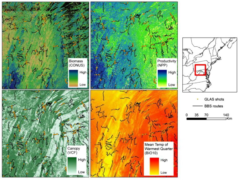
Figure 2. Maps showing BBS routes and GLAS shots overlaid on a sample of some of the predictor variables.
Download figure:
Standard image High-resolution image2.2.1. Random Forests
In Random Forests, we used 500 trees, each built using bootstrapped samples of the data and a randomly selected set of input variables, with an internal unbiased estimate of the generalization error produced (see appendix
2.2.2. Comparisons with USDA Forest Service bird distribution maps
To independently assess the validity of our predictions of species richness spatial distribution patterns, we compared our 1 km resolution maps with those from Matthews et al (2011) 20 km resolution maps (henceforth referred to as the USFS data set). They evaluated 147 breeding bird species across the eastern United States (Matthews et al 2007, 2011). We selected bird species they modeled with 'high reliability', including 53 species with habitat types that matched the breeding habitat guilds considered in our analysis. We note that Matthews et al (2011) only considered BBS data east of the 100th meridian from 1981 to 1990, whereas the BBS data we used span the entire contiguous US from 2004 to 2006 (inclusive).
The spatial data for each bird species in our maps were reclassified from predicted incidence values (the proportion of routes with species present on a scale from 0 to 1) to presence/absence cells. Species richness values (i.e. the number of bird species per cell) were generated for each guild and results were resampled to 20 km resolution to match the cell size and spatial extent of the USFS data set. Relative species richness was calculated for both data sets, multiplying each by 100 and dividing by the maximum species richness value present. We also compared the predicted habitat center for each guild, i.e. the latitude and longitude of the geographic center of each distribution, weighted by species richness. Lastly, we explored spatial correlations between the mapped data sets, showing where they agreed best and least. More specifics on the methodological approach are described in appendix
3. Results
3.1. Predictor variable correlations
The predictor variables most strongly correlated with bird species richness varied by guild type (figure 3). For total species richness vegetation property variables generally had the greatest predictive capability, followed by physical environment (e.g. temperature, precipitation) and canopy structure (see also appendix figure C.1). By guild, vegetation property variables typically had the highest correlations with species richness, with the exception of scrub birds (figure D.1). Considering environmental variables alone (see table 2), those most highly correlated with bird richness were also distinct for each guild. Temperature variables were most strongly correlated with forest bird richness, while precipitation variables were the strongest environmental correlates of open woodland bird richness (figure 3).

Figure 3. Correlation bar plots between predictor variables and species richness, for all birds and by guild. White bars indicate a negative and gray a positive correlation. Only significant correlations are shown (p < 0.05).
Download figure:
Standard image High-resolution imageThe correlation between vegetation properties, structure and bird richness were generally positive for the forest bird guild and negative for non-forest guilds (e.g. grassland). Conversely, the percent of grassland surrounding the route (lfgrass) showed a strong positive correlation for grassland bird richness whereas there was a negative correlation for forest birds (figure 3). Forest bird richness has the strongest correlations with the percent tree cover and also with EVI, percent area with mixed leaf longevity, and percent area with mixed leaf type. Open woodland bird richness was most correlated with EVI, percent area covered by deciduous trees, and percent area covered by broadleaf trees (figure 3). Scrub bird richness was most strongly correlated with bioclimatic variables rather than vegetation properties, although this result was probably influenced by the small range of scrub bird richness (between 0 and 11 species) in the BBS data set.
3.2. Prediction models
A combination of vegetation property and physical environment (i.e. climate variables) variables were the most influential predictors of species richness (figure 4). Bird species richness was predicted only moderately well for all guilds (R2 = 0.34) but the predictive models were strong for forest birds (R2 = 0.85) and moderately strong for the other guilds (R2 = 0.60−0.75). The most important variables for predicting forest bird richness were VCF and percent of BBS route area forested (LF tree). Grassland bird species richness was also well predicted by VCF and percent area forested, based primarily on strong inverse correlations of these predictions with richness. Open woodland species richness was most dependent on climatic variables, but also on biomass and VCF. Scrub bird models were the least robust, and only climate (primarily temperature) variables were important predictors.
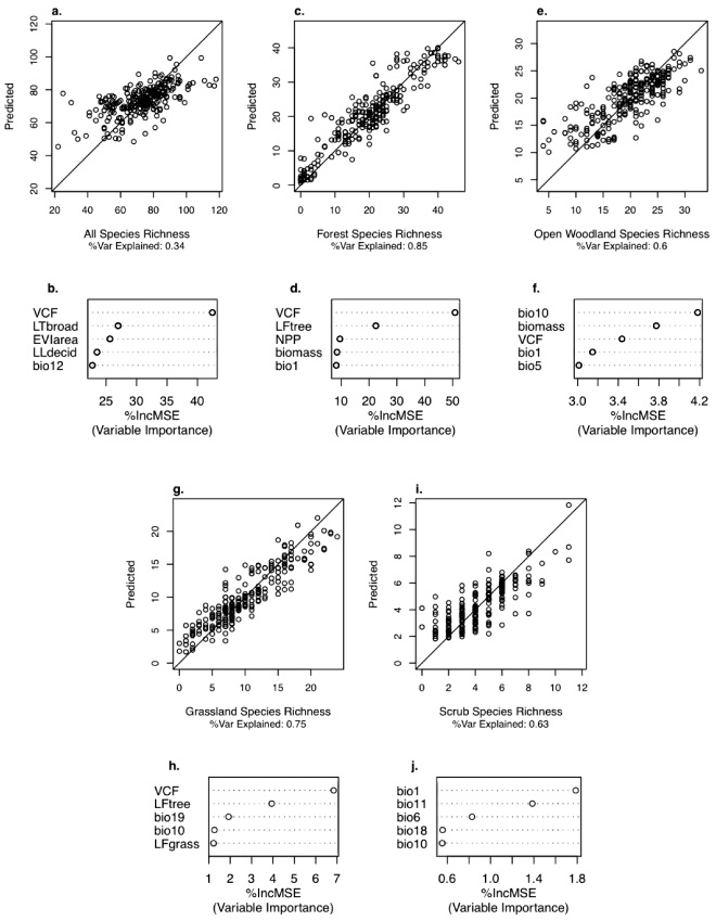
Figure 4. Cross validation results (upper panels: a, c, e, g, i) for the RandomForest models comparing reserved data values (X-axis) with the predicted model values (Y -axis). Variable importance plots (lower panels: b, d, f, h, j) show the percent increase in mean square error (%IncMSE), where higher values indicate model predicted values more similar to those observed.
Download figure:
Standard image High-resolution imageFurther partitioning the data set for forest birds and re-running random forest models for only those routes with high productivity (NPP > 550 gC m−2 yr−1) and high vegetation canopy cover (VCF > 50%) (figure E.1) allowed us to assess which predictor variables were most important for conditions that are more characteristic of densely vegetated, high productivity environments (figure 5). While climate variables were the most important predictors of forest bird richness in these environments, canopy structure metrics were also correlated (figure F.1). Compared to the entire set of forest birds, the species richness values were higher and restricted to a somewhat smaller range, but the cross-validated predictive models were still robust (R2 = 0.75 for both) (figures 5(a), (e)).

Figure 5. Cross validation results for forest birds in environments of high productivity (panel a) and high vegetation cover (panel e). Variable importance plots (panels b, f) are as in figure 4. Partial dependency plots (panels c, d, g, h) show the dependency of species richness (y-axis) on varying levels of the predictor variables independent of all other predictors.
Download figure:
Standard image High-resolution imageThe partial dependency plots in figure 5 show how predictor variables co-vary with the response variable (species richness) across their respective ranges. Notably, forest bird species richness in high productivity areas increased with biomass and canopy vertical complexity, particularly above the 20th percentile of both variables, but declined above the ∼20th percentile for all the selected climate variables. Similar results were observed for species richness in areas with high canopy cover (figure 5 lower panels), with declining richness above the ∼20th percentile for all climate variables and particularly rapid increases in richness up to the 40th percentile of biomass and the 50th percentile of vertical complexity values.
Additional partial dependency plots for all the guilds are presented in figure G.1. Notable trends include the systematic increase in forest bird richness with each of the most important predictor variables, the converse relationship for grassland birds (richness declines with increases in about half of the key predictors), and distinctly hump-shaped relationships for both open woodland and scrub birds (with highest species richness at mid-range values of the predictors). These observations were particularly evident for the canopy structure variables (right set of panels in figure G.1).
3.3. Bird species distributions and comparisons with USDA Forest Service maps
Maps of species richness derived from the BBS-route-based models (figure 6 right), and the continuous maps derived from the models being applied to the stack of spatial data layers (figure 6 left), both show coherent spatial patterns and strong regional gradients that vary by guild type. The route-based models and the continuous predictions show similar spatial patterns of richness, although the continuous maps reveal considerable spatial variability across the domain, with the highest total richness levels in the eastern US, particularly at higher latitudes. This pattern is even more pronounced for forest birds. High richness of open woodland birds spanned much of the eastern US as well, but was more widely distributed across the region. Grassland species richness, as expected, was particularly high in the west-central US We did not create maps of scrub birds owing to the less robust models for that guild.

Figure 6. Maps of species richness for all birds (top) and for three guild types (forest, woodland, grassland birds). The maps on the left represent the modeled distribution of species richness continuously across the study domain, each developed from the route-level models shown on the right and the suite of geospatial data layers (table 2).
Download figure:
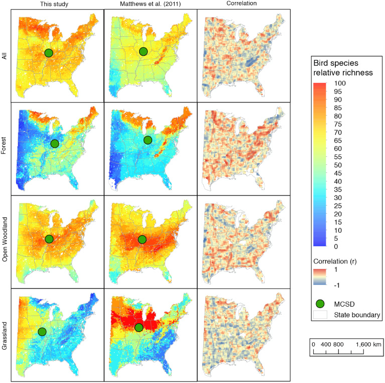
Standard image High-resolution imageOur predicted patterns of relative species richness correlate reasonably well with those of Matthews et al (2011). Overall, the weighted mean center of the species richness spatial distributions (see section 2.2.2) for our study and Matthews et al (2011) was geographically close for each guild type (figure H.1). They were closest for the open woodland guild (9.3 km) and farthest for the grassland guild (179.3 km). There was, however, considerable variability in the spatial correlation patterns. In both, forest bird richness was greatest around the Great Lakes, New England and the Appalachian Mountains. The spatial pattern comparison was least similar for grassland birds, with predictions from the USFS data set being high in the mid-western states and those from ours being concentrated further west. Both maps predicted the highest relative richness of open woodland species in the central eastern US, but the USFS data set predicted a larger expanse of high values.
4. Discussion
Our results show the various data sets (table 2) used in our analyses can inform models that robustly predict the spatial patterns of bird species richness across large areas, in this case the conterminous USA. While previous studies report similar findings at national (Coops et al 2009, Culbert et al 2013, Pidgeon et al 2007, Rittenhouse et al 2012) and regional scales (Allen and O'Connor 2000, Donovan and Flather 2002), we anticipated the influence of canopy structure captured in the lidar data sets would have greater predictive capability than we observed. This expectation was based on increasing evidence, using lidar-derived canopy structure measurements, that structure is an important predictor of species richness at local to regional scales (Bradbury et al 2005, Clawges et al 2008, Goetz et al 2010, 2007, Hill et al 2004, Lesak et al 2011, Seavy et al 2009, Swatantran et al 2012). Instead, our national scale estimates of forest bird guild species richness were most strongly influenced by tree canopy cover (i.e. VCF) and tree life form distribution (LFtree). Interestingly, we show robust predictions of forest bird richness even in areas of high productivity and high canopy cover, where we might expect some predictor variables to saturate in their sensitivity to increasing species richness, and canopy structure to become an important determinant of niche diversity. In these areas of high productivity and canopy cover, however, climate variables became important predictors (figure 5), indicating they capture additional information beyond even integrative variables like net primary production. In the case of woodland birds, a unimodal shape of the partial dependency plots reflects greatest species richness at intermediate vegetation cover, biomass and canopy structure values. This finding is consistent with greater landscape habitat diversity in more open woodland areas relative to, e.g. densely forested or open grasslands areas, and expectations of different woodland bird species utilizing differing vegetation types and densities.
The predicted patterns of relative species richness from our models were generally similar to those Matthews et al (2011) mapped for the eastern US, even though very different approaches were used to generate the maps produced by both studies. There are several differences worth noting. First, although both studies considered climate, elevation, and tree species properties as predictor variables, the other predictors differed substantially between the two studies. In particular, our predictions considered unique vegetation properties (e.g. biomass, productivity) and canopy structure metrics (e.g. canopy height, vertical complexity). We note these were aggregated to coarser resolution (20 km) for comparison with the Matthews et al (2011) maps. In addition, the BBS data sets used in this study and the USDA Forest Service maps were collected more than a decade apart. We expected this to adversely impact the comparison insofar as the time lag might contribute to changes in bird species richness and/or the predictor variables, but the overall similarities between the relative richness maps was an encouraging confirmation of the utility of our higher resolution predicted richness distribution maps (figure 6). This was particularly true given we used only what Matthews et al (2011) deemed their highest quality species predictions (appendix
These points noted, the strength of any predictor variable is fundamentally related to the scale at which the metric is most ecologically relevant. Our models tended to characterize forest vegetation type, cover and climate as the most important large area predictors of bird species richness, despite the considerable influence of canopy structure at more local scales. However, the inability of sample sets of 70 m GLAS lidar shots to fully characterize entire 40 km BBS routes complicates these interpretations. Canopy structure can undergo significant changes over the length of the route, and averaging all shots intersecting a route probably does not represent conditions of the entire route. A more direct analysis of bird observations within the footprint of the GLAS shots would better capture the attributes of bird species richness that are dependent on canopy structure and related habitat heterogeneity, but the BBS data were not collected with that intent (i.e. data are aggregated for all stops along the length of the routes). This does not mean that very large-scale studies of habitat structure with lidar are impractical, but it is important to note that GLAS lidar are samples (not wall-to-wall images). Despite that, we found meaningful correlations between GLAS structure metrics and bird species richness when compared in a pairwise manner (figures E.1, F.1). Moreover, the partial dependency plots (figure G.1) show reasonable and expected associations of structure metrics with forest birds (positively co-varying), woodland birds (richness peaking at intermediate values of structure metrics) and even grassland birds (negatively co-varying). Previous work with airborne lidar shows more densely sampled lidar structure metrics are useful for predicting not only richness but habitat use, thus future studies of the relative importance of species richness predictors might explore the effect of spatial averaging of structural variability that accompanies increasing lidar footprint size, as well as sampling density and terrain-influenced height estimation errors in medium to large footprint lidar systems. Such studies would be best designed in the context of potential next generation space-borne lidar systems relevant to vegetation and ecosystem studies.
Acknowledgments
We thank Steve Matthews (USDA Forest Service) for providing his maps of bird species distribution for the eastern United States, Kevin Guay for assistance with statistical comparisons, and the BBS staff and volunteers for making their data widely available. This work was supported by the NASA Applied Sciences (Biodiversity) program managed by Woody Turner (grant NNX09AK20G).
Appendix A.: Additional information on methodological approach
Lidar metric derivation. In deriving lidar metrics, we eliminated shots that did not produce adequate waveforms (e.g. shots with excessive atmospheric attenuation including clouds), specifically shots where the amplitude of the raw waveform does not exceed twice the noise threshold. We also excluded shots in which the waveform contained less than two distinct peaks (an indication that the top of the vegetation canopy was not detected), as well as shots in areas with substantial topographic relief, where canopy height estimation was problematic (Lefsky et al 2007). A total of 48,133 GLAS shots remained post screening, which was less than half of the total number of shots acquired and processed.
Random Forests models. We subsequently applied the lidar (i.e. structural information), physical environment, and vegetation properties metrics in Random Forests to assess predictor variable importance. In Random Forests, data are partitioned using a series of hierarchical binary splits on the predictor variables, with the goal of maximizing explained variance in the response variable (in our case bird species richness). A different bootstrapped random sample of the data for each tree is used to optimally split among the various predictors, improving performance by iteratively aggregating the results. Predictors are selected randomly, which acts to increase the accuracy of the model while reducing the influence of variable selection order and, in the process, minimize overfitting (Cutler et al 2007). The combined effects of the predictor variables were assessed using the mean prediction of many individual regression trees.
Generation and comparison of relative richness maps. Species presence/absence thresholds were optimized by Matthews et al (2011), who found an optimal incidence value (IV) cutoff at 0.05 (i.e. grid cells with IV < 0.05 were reclassified as zero, indicating species absence). We subsequently explored the regional correlations between our model predictions (figure 5) and those of Matthews et al (2011) through maps of spatial correlation, which we created by writing a moving window script that derived a regression model for the cell values (from both data sets) within the same 5 × 5-cell window and created a new map with the correlation coefficient in the window centroid. The window iterated across both data sets, producing maps of the spatial correlation between the data sets. The moving window assigned null values in regions where identical richness values (in either or both data sets) populated a 5 × 5 window because the standard deviation in these cases was zero. Relative species richness was calculated for both data sets, multiplying each by 100 and dividing by the maximum species richness value present. We also compared the predicted habitat center for each guild by calculating the mean center of spatial distribution, weighted by species richness (using the Mean Center tool).
Appendix B:
See table B.1.
Table B.1. Bird species with high model reliability from the USDA Forest Service Climate Change Bird Atlas (www.nrs.fs.fed.us/atlas/bird) (Matthews et al 2007). Guild classifications were based on the Cornell Lab of Ornithology habitat type classifications.
| Common name | Scientific name | Guild |
|---|---|---|
| Tufted Titmouse | Baeolophus bicolor | Forest |
| Purple Finch | Carpodacus purpureus | Forest |
| Veery | Catharus fuscescens | Forest |
| Black-billed Cuckoo | Coccyzus erythropthalmus | Forest |
| Black-throated Blue Warbler | Dendroica caerulescens | Forest |
| Yellow-rumped Warbler | Dendroica coronata | Forest |
| Magnolia Warbler | Dendroica magnolia | Forest |
| Pine Warbler | Dendroica pinus | Forest |
| Wood Thrush | Hylocichla mustelina | Forest |
| Red-bellied Woodpecker | Melanerpes carolinus | Forest |
| Rose-breasted Grosbeak | Pheucticus ludovicianus | Forest |
| Black-capped Chickadee | Poecile atricapillus | Forest |
| Ovenbird | Seiurus aurocapillus | Forest |
| Red-breasted Nuthatch | Sitta canadensis | Forest |
| Brown-headed Nuthatch | Sitta pusilla | Forest |
| Yellow-bellied Sapsucker | Sphyrapicus varius | Forest |
| Winter Wren | Troglodytes troglodytes | Forest |
| Nashville Warbler | Vermivora ruficapilla | Forest |
| Red-eyed Vireo | Vireo olivaceus | Forest |
| White-throated Sparrow | Zonotrichia albicollis | Forest |
| Northern Bobwhite | Colinus virginianus | Grassland |
| Bobolink | Dolichonyx oryzivorus | Grassland |
| Horned Lark | Eremophila alpestris | Grassland |
| Savannah Sparrow | Passerculus sandwichensis | Grassland |
| Ring-necked Pheasant | Phasianus colchicus | Grassland |
| Dickcissel | Spiza americana | Grassland |
| Common Ground-Dove | Columbina passerina | Scrub |
| Common Yellowthroat | Geothlypis trichas | Scrub |
| Yellow-breasted Chat | Icteria virens | Scrub |
| Painted Bunting | Passerina ciris | Scrub |
| Clay-colored Sparrow | Spizella pallida | Scrub |
| Field Sparrow | Spizella pusilla | Scrub |
| White-eyed Vireo | Vireo griseus | Scrub |
| Cedar Waxwing | Bombycilla cedrorum | Open woodland |
| Chuck-Will's Widow | Caprimulgus carolinenis | Open woodland |
| Northern Cardinal | Cardinalis cardinalis | Open woodland |
| American Goldfinch | Carduelis tristis | Open woodland |
| Hermit Thrush | Catharus guttatus | Open woodland |
| Yellow-billed Cuckoo | Coccyzus americanus | Open woodland |
| Yellow Warbler | Dendroica petechia | Open woodland |
| Gray Catbird | Dumetella carolinensis | Open woodland |
| Blue Grosbeak | Guiraca caerulea | Open woodland |
| Baltimore Oriole | Icterus galbula | Open woodland |
| Orchard Oriole | Icterus spurius | Open woodland |
| Loggerhead Shrike | Lanius ludovicianus | Open woodland |
| Red-headed Woodpecker | Melanerpes erythrocephalus | Open woodland |
| Song Sparrow | Melospiza melodia | Open woodland |
| Indigo Bunting | Passerina cyanea | Open woodland |
| Summer Tanager | Piranga rubra | Open woodland |
| Chipping Sparrow | Spizella passerina | Open woodland |
| Carolina Wren | Thryothorus ludovicianus | Open woodland |
| House Wren | Troglodytes aedon | Open woodland |
| American Robin | Turdus migratorius | Open woodland |
Appendix C:
See figure C.1.

Figure C.1. Boxplot of the correlation (absolute value) between predictor variables and species richness, by variable class, for the model predicting richness of all birds (i.e. aggregated guilds).
Download figure:
Standard image High-resolution imageAppendix D:
See figure D.1.

Figure D.1. Dotplots showing the correlation range of the ten strongest predictor variables by bird guild and organized by predictor variable class. Open dots indicate negative correlation and solid dots positive correlation. An empty line indicates no predictor variables in that class were among the ten most important for predicting species richness.
Download figure:
Standard image High-resolution imageAppendix E:
See figure E.1.

Figure E.1. Maps showing the location of BBS routes with high NPP (left panels) and high VCF (right panels) for all routes where forest birds were dominant in terms of species richness (top panels) or simply present (bottom panels). Colors indicate magnitude of forest bird species richness.
Download figure:
Standard image High-resolution imageAppendix F:
See figure F.1.
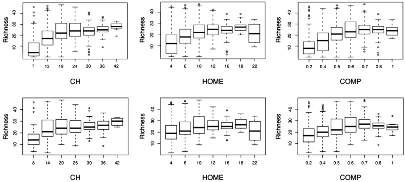
Figure F.1. Boxplots showing the relationship between species richness of all birds (top panels) and forest birds (bottom panels) relative to selected canopy structure variables in areas of high NPP. The forest bird richness panels correspond to the routes in figure E.1 where forest birds were dominant.
Download figure:
Standard image High-resolution imageAppendix G:
See figure G.1.
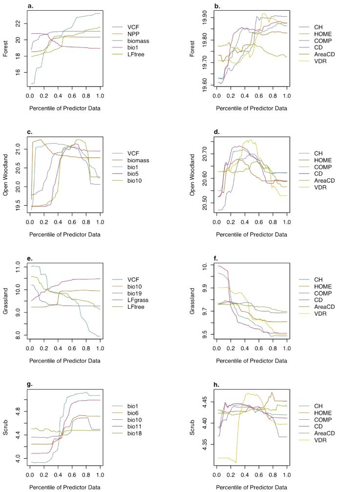
Figure G.1. Partial dependency plots for each bird guild type, with the most important predictors shown at left and canopy structure metrics at right.
Download figure:
Standard image High-resolution imageAppendix H:
See figure H.1.
Figure H.1. Relative richness maps from bird species model outputs of this study (left images) and Matthews et al (2011) (middle images), and the correlation between the two data sets (right images). Green dots in the relative richness maps indicate the mean geographic center of distribution (MCD) for all birds and each guild type. White areas within the eastern US in the correlation maps indicate null value regions (see appendix A).
Download figure:
Standard image High-resolution image