
Abstract
A new vegetation trend is emerging in northeastern forests of the United States, characterized by an expansion of red maple at the expense of oak. This has changed emissions of biogenic volatile organic compounds (BVOCs), primarily isoprene and monoterpenes. Oaks strongly emit isoprene while red maple emits a negligible amount. This species shift may impact nearby urban centers because the interaction of isoprene with anthropogenic nitrogen oxides can lead to tropospheric ozone formation and monoterpenes can lead to the formation of particulate matter. In this study the Global Biosphere Emissions and Interactions System was used to estimate the spatial changes in BVOC emission fluxes resulting from a shift in forest composition between oak and maple. A 70% reduction in isoprene emissions occurred when oak was replaced with maple. Ozone simulations with a chemical box model at two rural and two urban sites showed modest reductions in ozone concentrations of up to 5–6 ppb resulting from a transition from oak to red maple, thus suggesting that the observed change in forest composition may benefit urban air quality. This study illustrates the importance of monitoring and representing changes in forest composition and the impacts to human health indirectly through changes in BVOCs.
Export citation and abstract BibTeX RIS

Content from this work may be used under the terms of the Creative Commons Attribution 3.0 licence. Any further distribution of this work must maintain attribution to the author(s) and the title of the work, journal citation and DOI.
1. Introduction
For more than a century, a dramatic change has been observed in forests in the eastern United States resulting in a rapid increase in the density of red maple (Acer Rubrum) at the expense of a variety of oak species (Quercus) (Larson 1953, Lorimer 1984, Abrams 1992, 1998, Nagel et al 2002). The magnitude of change depends on location and composition of oak species, but ranges from as little as 10% to more than a 70% reduction of oaks over the last century (Abrams 1998, 2005). The shift in species composition has been attributed to land use change, particularly land management practices related to fire suppression, grazing, and logging (Lorimer 1984, Abrams 1992, 1998). Before and during the early settlement period in the United States, prescribed burns were performed to remove brush and debris in the understory of forests. This practice has allowed oak species to thrive while forcing red maple to retreat into wetland regions, as oak are resistant to fire (Abrams 1992), while red maple is highly vulnerable (Abrams 1998). As new land management practices have shifted away from prescribed burns, red maple can easily out-compete oak species for available light, moisture, and nutrients (Abrams 1998). Furthermore, because red maple can survive in a large range of environments, it is considered an early and late successional species (Abrams 1998). If the observed trend continues as expected, many eastern forests will be void of historically dominant oaks, perhaps as soon as the end of this century (Abrams 1998, 2005).
While there are numerous ecosystem services provided by oak-dominated forests, they are also high emitters of biogenic volatile organic compounds (BVOCs), including isoprene (C5 H8) and monoterpenes (C10 compounds). In regions of anthropogenic pollution, high isoprene can favor the production of ozone leading to smog formation and poor air quality. Therefore, a restructuring of the composition of eastern forests may in fact benefit the air quality of urban areas because of differences in the amount of BVOC emissions between the two species The difference in BVOC emissions between red maple and oak is quite large; oak species emit approximately 98% more isoprene than red maple (Hewitt et al 2005) Furthermore, it has been shown that changes in species composition within a forest might have a greater impact on isoprene emissions than changes in forest area (Purves et al 2004). Because BVOCs are precursors for ozone formation, a decrease in BVOC emissions could lead to a decrease in ozone in regions with high concentrations of nitrogen oxides (NOx) (Sillman 1999). Isoprene and other VOCs can be oxidized by hydroxyl (OH) radicals (with a lifetime of 1.4 h (Warneck and Williams 2012)) to form peroxy (RO2) radicals, which react with NO to generate NO2. The photodissociation of NO2 then leads to ozone formation. Additionally, some isoprene oxidation pathways can lead to the formation of secondary organic aerosols (e.g., Claeys et al 2004). Monoterpenes are emitted in lower quantities than isoprene and play a lesser role in ozone formation, but are important for the formation of secondary organic aerosols (Griffin et al 1999). Because BVOCs exceed anthropogenic VOCs in some regions, it is often more difficult to control VOC emissions than anthropogenic NOx (Lin et al 2005, Aksoyoglu et al 2012) The ecological shift towards the dominance of red maple species may reduce biogenic isoprene emissions and contribute to lower ozone concentrations. Therefore, the expansion of red maple could aid in the air quality of forested urban centers undergoing this change.
Because of the deleterious effects of ozone on human health and ecosystems, the US Environmental Protection Agency (EPA) established the National Ambient Air Quality Standards (40 CFR Part 50, FR62 38856) for six criteria pollutants, including ozone. The current recommended ozone concentration is less than 0.075 parts per million (ppm) averaged over 8 h; however, the EPA has proposed lowering this to 0.06–0.07 ppm (40 CFR Part 50 and 58, FR75 2938). Regions with ozone concentrations higher than these guidelines (classified as nonattainment) would be required to take action to reduce ozone precursor emissions. As of 2013, over 120 counties in the northeastern region (figure 1) were classified as marginal to moderate nonattainment in whole or partial county areas (www.epa.gov/ozonedesignations) and an additional 131 counties were classified as maintenance areas. Numerous studies have documented an overall increase in the concentration of ozone in regions with existing NOx emissions when an increase of isoprene was detected (Roselle 1994, Pierce et al 1998). Control strategies for decreasing ozone should consider reductions in both VOCs and NOx; however the most beneficial control strategy is dependent on the amount of local BVOCs (Roselle 1994), and understanding how species succession affects BVOC emissions can assist in evaluating potential control strategies where land cover change is occurring.
In this study, we consider changes in the Northeastern United States forest composition resulting from the expansion of red maple and concomitant decline of oak. We investigate changes in summertime BVOC emissions and resulting ozone concentrations in three theoretical forest composition cases relative to a baseline case representing present day land cover and climate conditions. These three cases reflect both extreme conditions of conversion to an all red maple forest or an all oak forest as well as one intermediate scenario meant to capture partial conversion that has already been documented in some eastern forests. We use the Global Biosphere Emissions and Interactions System (GloBEIS; Yarwood et al (1999)) to simulate BVOC emissions of isoprene and monoterpenes along with a 0D photochemical box model (Silman 1991) to simulate how changes in these biogenic emissions will affect the production of ozone in both urban and rural areas
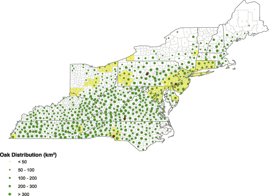
Figure 1. Density of oak trees in the northeastern United States according to the BELD3 dataset. Each dot represents the oak tree distribution within a county. Regions in yellow represent counties that are considered in ozone nonattainment by the EPA. Red diamonds represent locations where the chemical box ozone model was run.
Download figure:
Standard image High-resolution image2. Methods
2.1. GloBEIS model description
GloBEIS was developed to simulate BVOC emissions for 230 vegetation species over a wide range of temporal scales and regions (Yarwood et al 1999). The model produces emission inventories for isoprene, monoterpenes and other VOC based on input climate data (e.g., temperature, precipitation, cloud cover) with some flexibility in specifying other vegetation parameters for the purposes of sensitivity testing. GloBEIS has been evaluated versus ground-based observations for Texas (Yarwood et al 1999), central Africa (Guenther et al 1999), and North America (Guenther et al 2000).
GloBEIS was used in this study because it uses vegetation species-specific emissions factors, it requires minimal inputs, and it can be run on a desktop computer. The emission factors used in GloBEIS are the same as those reported by Guenther et al (1995) and the MEGAN model, but expressed at the leaf level and not the canopy level; although the canopy emission factors used in MEGAN are largely derived from branch and leaf enclosure data extrapolated to the whole canopy (Guenther et al 2006). Overall, isoprene emissions between GloBEIS and MEGAN are comparable (Sakulyanontvittaya et al 2010). Current modeling methods are limited by data availability of emission factors and estimations of land cover, as well as projections of future land cover change. Guenther et al (2000) estimated uncertainty in biogenic emission estimates to be around a factor of 3. Furthermore, many studies estimate vegetation cover from broad-based biomes and estimate biogenic emissions from an average flux over the land cover type, and variations within the biome can account for some uncertainty in estimated emissions. However, because most BVOC models yield similar isoprene emissions (Arneth et al 2008), GloBEIS is an appropriate model for this study.
GloBEIS calculates emissions similar to Guenther et al (2000) as well as the more recent MEGAN model (Guenther et al 2006, 2012) with

where ε is the emission rate at the leaf level for a specific vegetation type at standard temperature and level of photosynthetically active radiation (PAR), D is the foliar density, and ϒ is an activity factor accounting for deviations in the standard of photon flux density, temperature, and leaf age, ρ accounts for loss within plant canopies and A is the area of the vegetation species. Additional emission factors (e.g., leaf age, prior light and temperature history) in MEGAN are not included in GloBEIS, yet these generally make minor adjustments to emissions and most isoprene models estimate similar magnitudes of emission (Arneth et al 2008). For this study we use leaf level isoprene emission factors of 0.1 μg C g−1 h−1 for red maple and 70 μg C g−1 h−1 for oak species, and monoterpene factors of 1.6 μg C g−1 h−1 for red maple and 0.2 μg C g−1 h−1 for oak species (Geron et al 1994) The options for variable LAI, variable leaf age, and drought index were not used and ρ was set to 1. Because variability of isoprene emissions is dependent on changes in temperature and PAR, our use of constant atmospheric forcing for all scenarios results in changes to the emission rate and area of the vegetation species.
2.2. BVOC modeling
GloBEIS is driven with 6-hourly climate input from the National Center for Environmental Protection (NCEP) reanalysis dataset (Kalnay et al 1996) that includes temperature, photosynthetically active radiation, wind speed, and humidity at a spatial resolution of 0.5° for the period 1990–1999. The vegetation distribution is derived from version 3 of the Biogenic Emissions Landuse Dataset (BELD3) and represents land use of the 1990s at a 1 km resolution (Kinnee et al 1997). The BELD dataset was designed for use in the EPA's BEIS model (Biogenic Emissions Inventory System), which can be used in the GloBEIS framework. Each cell is assigned a vegetation biome, with information about the fraction of forest, agriculture, and other land cover type (e.g., water, urban built-up). Species information is provided for 230 vegetation types including trees and crops as a fraction of the total area in each county (ftp://ftp.epa.gov/amd/asmd/beld3).
Our chosen domain includes 17 states (figure 1) where forest surveys show an increase in red maple and a decrease in oak (Christensen 1977, Russel 1980, Ross et al 1982, Lorimer 1984, Abrams et al 1995, Abrams 1998, Dyer 2001, Abrahamson and Gohn 2004, Abrams 2005, Galbraith and Martin 2005). The dominant tree species in the domain is oak (almost 13% of the total area) followed by red maple (less than 5%). We created a land cover file from the BELD3 dataset for each county in the domain, allowing the resolution of the model to vary depending on the size of the county. The top 20 land cover types account for 85% of the total land cover in the domain (table 1).
Table 1. Area (km2) and percent of total area of the 21 dominant land cover types found in the northeastern United States domain as defined in the BELD3 dataset (Kinnee et al 1997). Total area of the model domain is 1057 059.2 km2.
| Land cover type | Area (km2) | Per cent of total area |
|---|---|---|
| Quercus (oak) | 13 6676.1 | 12.9 |
| Water | 94 568.5 | 8.9 |
| Acer (all maple except red maple) | 33 787.9 | 3.2 |
| Acer Rubrum (only red maple) | 48 919.0 | 4.6 |
| Miscellaneous crop | 156 168.1 | 14.8 |
| Mixed forest | 49 174.1 | 4.7 |
| Pinus (pine) | 48 364.6 | 4.6 |
| Corn | 43 476.5 | 4.1 |
| Hay | 39 459.7 | 3.7 |
| Fagus (beech) | 34 321.5 | 3.2 |
| Soybeans | 33 366.0 | 3.2 |
| Carya (hickory) | 29 500.8 | 2.8 |
| Cornus (dogwood) | 20 831.6 | 2.0 |
| Betula (birch) | 20 764.2 | 2.0 |
| Ulmus (elm) | 19 370.2 | 1.8 |
| Fraxinus (ash) | 17 969.5 | 1.7 |
| Liriodendron (tulip poplar) | 17 475.4 | 1.7 |
| Deciduous forest | 16 824.6 | 1.6 |
| Prunus (cherry) | 15 206.1 | 1.4 |
| Sassafras | 12 933.6 | 1.2 |
| Abies (fir) | 12 619.9 | 1.2 |
| Total | 901 776.93 | 85.3 |
We performed a baseline run (BASELINE) using present day vegetation cover from BELD3 and a set of three theoretical land cover change experiments. To isolate the isoprene emission signal resulting from the imposed land cover changes alone, all model runs were driven with the same NCEP climate data. In the first theoretical experiment, all oak species were removed and replaced with red maple (MAPLE). In the second experiment, all red maple were removed and replaced with oak (OAK) to obtain an upper limit of isoprene emissions that may have existed in the past. One additional experiment was conducted to assess how isoprene changes with fractional land cover changes (e.g., 50% replacement of oak versus 100% replacement) that have been documented in some eastern forests. In this experiment, 50% of the oaks were converted to red maple (50%OAK2MAPLE).
2.3. Ozone modeling
We tested the sensitivity of ozone formation to land cover change-driven BVOC emissions changes using a 0D photochemical box model based on Silman (1991). While 3D chemical transport modeling would be ideal to investigate the full chemical impact of these ecosystem changes, the 0D model provides a first estimate of the relative impact of the biogenic VOC changes at specified locations. The 0D model treats each location as a single 'box' and assumes a constant wind speed of 2 m s−1 to represent dilution due to horizontal advection along with prescribed upwind and downwind concentrations, providing a simple estimate of transport based on current land cover. Initial and advected model concentrations were derived from July climatological (2000–2007) global chemistry model simulations (MOZART; (Emmons et al 2010); ∼2.8° by 2.8° or T42 spatial resolution) for ozone, CO, NOx, and a suite of anthropogenic VOC species. The height of the box is prescribed with a diurnally evolving mixed height layer from 150 m at night to 1500 m at midday to mimic the diurnal dilution of pollutants in the boundary layer. Explicit vertical mixing is not included, although a top boundary condition is specified based on the global MOZART concentrations A diurnal temperature range of 20 K from daily minimum to maximum is the same for all locations. Regional ozone formation can also be affected by the formation and transport of isoprene nitrates (Fiore et al 2005) but we have not considered the transport of these compounds in this study.
Emissions input to the box model are based on theMACCity global 0.5° resolution database (Lamarque et al 2010) and include emissions of NOx, CO and anthropogenic VOC. BVOC emissions were derived from the GloBEIS simulations as described in section 2.2. The box model uses the GEOS-Chem mechanism modified for urban photochemistry (Evans et al 2003, Ito et al 2007) and treats isoprene chemistry explicitly and monoterpene chemistry with two surrogates (one as α-pinene and one as limonene), which have OH lifetimes of 2.7 h and 51 min, respectively; (Warneck and Williams 2012). We assume a 50–50 split of monoterpene emissions to these two categories, though note that there can be significant variability of the monoterpene speciation of emissions depending on the vegetation type (Geron et al 2000). Generally, the monoterpene emission quantities and changes are relatively small compared to the isoprene and have a smaller impact on ozone formation, therefore the following sections focus on isoprene emissions and their effects on ozone.
We selected four geographic locations based on the following criteria: (1) the ozone attainment status, (2) the photochemical sensitivity, (3) the baseline biogenic VOC emissions, and (4) the emissions change due to land cover changes. The four locations are (1) the Philadelphia metropolitan area (39.9°N, 75.3°W), a suburban/urban region in non attainment for ozone with low baseline BVOC emissions and relatively low capacity for maple expansion, (2) the Charlotte metropolitan area (35.2°N, 80.9°W), a suburban/urban region in non-attainment for ozone with high baseline BVOC emissions and a high capacity for maple expansion, (3) western Virginia (37.2°N, 80.4°W), a rural site in attainment for ozone with high baseline emissions and a high capacity for maple expansion, and (4) central Pennsylvania (40.8°N, 77.9°W), a rural site in attainment for ozone with moderate BVOC emissions and a relatively low capacity for maple expansion.
Table 2. Comparison of estimated isoprene emission rates from select regional modeling studies and this study.
| Region | Isoprene emissions (Tg C yr−1) | Citation |
|---|---|---|
| North America | 29.3 | (Guenther et al2000) |
| United States | 15.5 | (Guenther et al2000) |
| United States | 22.05 | (Guenther et al1995) |
| United States | 29.1 | Lamb et al (1993) |
| EPA Region 3 (PA, DE, MD, VA, WV) | 2.1 | Lamb et al (1993) |
| Northeastern US | 3.18 | This study; current vegetation distribution (BASELINE) |
| Northeastern US | 0.98 | This study; all red maple (MAPLE) |
| Northeastern US | 3.81 | This study; all oak (OAK) |
| Northeastern US | 2.06 | This study; 50% oak to red maple (50% OAK2MAPLE) |
3. Results
3.1. Regional changes in BVOC emissions
For the BASELINE experiment, the average total isoprene emissions over the domain from 1990 to 1999 are 3.18 Tg C yr−1 (table 2). Direct comparison of our results with other studies is difficult because of the selected domain, which accounts for less than 12% of the continent. Total simulated isoprene emissions reported in this study are the same order of magnitude but slightly lower as those reported by Lamb et al (1993) covering just the Mid-Atlantic EPA Region 3 (table 2). Simulated July daily isoprene emissions range from a low of 4to8 mg C m−2 day−1 in the northern part of the domain to nearly 100 mg C m−2 day−1 in Virginia, North Carolina, and Tennessee (figure 2(a)) where oak density is highest along the Appalachian Range (figure 1). Regions with low concentrations of oak, such as Maine, New York, and Vermont do not show substantial isoprene emissions.
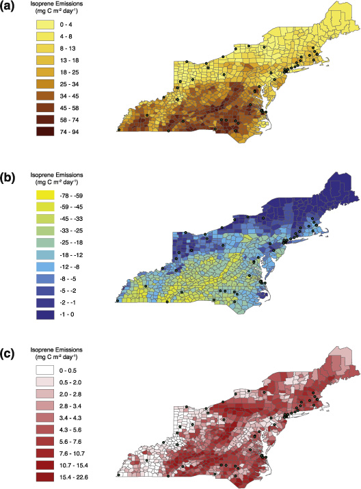
Figure 2. GloBEIS simulated average isoprene emissions (mg C m−2 day−1) for the month of July over the 1990–1999 period. (a) BASELINE case. (b) Change (MAPLE minus BASELINE) resulting from red maple replacing oak species. (c) Change (OAK minus BASELINE) resulting from oak species replacing red maple. Green dots represent cities with a population greater than 100 000.
Download figure:
Standard image High-resolution imageGloBEIS predicts a ∼70% decrease in isoprene emissions in the MAPLE simulation (table 2). Isoprene emissions decrease by more than 50 mg C m−2 day−1, especially in the southern part of the domain where the greatest density of oak was replaced (figure 2(b)) In contrast, isoprene emissions increase in the OAK simulation by approximately 20% over the entire domain (table 2). July daily emissions increased by more than 10 mg C m−2 day−1 with the largest increases concentrated along the Appalachian Mountains and in Massachusetts, New Hampshire, Rhode Island, and Connecticut (figure 2(c)). When a less dramatic land cover change of 50% conversion of oak to maple is imposed, the model simulates a 35% decrease in isoprene emissions in the 50% OAK2MAPLE scenario (table 2).
3.2. Impacts of BVOC changes on air quality
Major metropolitan areas (identified as those with a population greater than 100 000; figure 2) located in proximity to high isoprene emissions have a greater potential for ozone production. While most major cities are located in regions of relatively low isoprene emissions, several near the Appalachian Mountains have high isoprene emissions, particularly in North Carolina and Tennessee. Eighty six percent of the cities plotted are in counties of nonattainment of the EPA's 8-h ozone standard (figure 1). Depending on the prevailing wind direction, transport of isoprene downwind of high-density oak regions could impact air quality in surrounding areas, assuming that NOx is not a limiting factor.
Table 3 and figure 3 describe the impacts of BVOC emissions changes as simulated by the 0D photochemical box model in the four locations for the BASELINE and three land cover change scenarios. In all simulations, isoprene emissions are largest at the Western VA and Charlotte sites because they are in the southern portion of the domain where oak density is highest (figures 1 and 3). We compare the BASELINE modeled diurnal cycle of ozone with that observed at EPA Photochemical Assessment Monitoring Stations (PAMS) in each of the four locations (an average July diurnal cycle based on data from PAMS data from 1994–2010; (EPA 2011)).
Table 3. Ozone box model location descriptions and BASELINE model simulation details. Observed BASELINE NOx emissions obtained from the MACCity inventory (Lamarque et al 2010) and observed daily maximum ozone obtained from the EPA PAMS stations in each of the four locations (1994-2010 average; (EPA 2011)).
| Charlotte | Philadelphia | Central PA | Western VA | |
|---|---|---|---|---|
| Location type | Urban | Urban | Rural | Rural |
| Latitude | 35.2°N | 39.9°N | 40.8°N | 36.8°N |
| Longitude | 80.9°W | 75.3°W | 77.9°W | 79.9°W |
| Baseline isoprene emissions mg C m−2 h−1 | 4.91 | 0.01 | 8.16 | 3.60 |
| Baseline monoterpene emissions mg C m−2 h−1 | 0.42 | 0.05 | 0.82 | 0.15 |
| Baseline NOx emissions 1012 molec cm−2 s−1 | 27.3 | 52.5 | 7.69 | 8.13 |
| July observed ozone daily maximum (ppb) | 66 | 64 | 55 | 59 |
| Modeled ozone daily maximum (ppb) | 70 | 74 | 64 | 71 |
In general, the box model reproduces the diurnal cycle of ozone although it tends to overestimate the daily maximum by about 5–10 ppb in urban areas, and about 15 ppb in rural areas (figure 4). While this overestimation may influence our understanding of local air quality, these biases are typical for photochemical models in the Northeastern USA (Fiore et al 2009, Reidmiller et al 2009).
The large decrease in isoprene emissions in the MAPLE scenario yields the most substantial ozone reductions at three of the four sites (figure 4). In Philadelphia, the model is not sensitive to any of the changes in BVOC emissions, highlighting the small role of BVOCs in this region and the NOx-sensitivity of this location. In Charlotte, the 100% conversion of oak to maple leads to a 4 ppb reduction in the daily ozone maximum, and a 2 ppb reduction under the 50% conversion case (50% OAK2MAPLE). The effects on ozone are even stronger in the two rural sites, with an ozone reduction of up to 6 ppb in western VA. This suggests that the oak to maple transition may have greater impacts on rural regional ozone concentrations rather than within urban cores.
The OAK simulation predicts slight increases in isoprene emissions (figure 3(a)) accompanied by small decreases in monoterpene emissions (figure 3(b)). In Charlotte and Philadelphia, the OAK simulation shows almost no impact on ozone (<0.1 ppb increase) because of the relatively large amounts of anthropogenic VOC emissions (figure 4). In the rural areas where anthropogenic sources are much smaller, slight increases in isoprene emissions in the OAK scenario have a larger impact and lead to increases in daily maximum ozone concentrations of 1–3 ppb.
At all locations, changes in monoterpenes have little impact on ozone formation. While monoterpenes increase in the MAPLE scenario by about 20% at the southern sites and nearly double at the central PA site, the relatively low magnitude of monoterpene emissions and their lower ozone formation potential result in no significant impact on ozone production at the four sites.
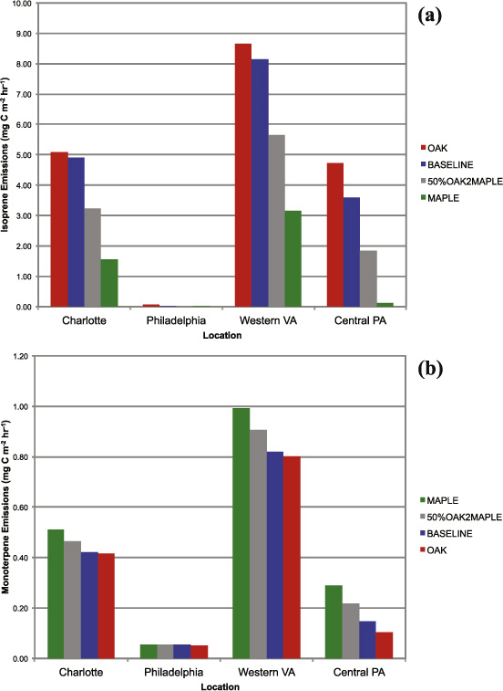
Figure 3. Maximum midday (a) isoprene emissions (mg C m−2 h−1) and (b) monoterpene emissions (mg C m−2 h−1) and (b) used for ozone box model land cover simulations.
Download figure:
Standard image High-resolution image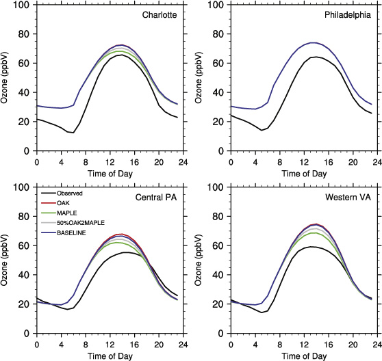
Figure 4. Average diurnal cycle of observed (black) and modeled O3 (ppbv) at four locations for the BASELINE case and the three land cover sensitivity experiments.
Download figure:
Standard image High-resolution image
4. Discussion and conclusions
The future composition of forests may have an unexpected effect on atmospheric chemistry and air quality. The MAPLE scenario, representing a future point in time when most of eastern forests may be void of oak, predicted a 70% decrease in isoprene emissions from BASELINE because of the low isoprene emission factors of red maple. Alternatively, a hypothetical scenario in which no red maple exist, predicted a 20% increase in isoprene emissions This species shift has the potential to reduce biogenic hydrocarbon emissions and improve the oxidation capacity of the atmosphere. These emissions changes varied regionally, with MAPLE predicting a 60–70% decrease in isoprene emissions in the south, a 100% decrease in central PA, and no change in Philadelphia. In contrast, the OAK scenario predicted a 3–6% increase in isoprene emissions in the southern locations and a 30% increase in central PA. Monoterpene emissions increased in proportion to the isoprene reductions, however, their relative contribution was minimal in the formation of ozone. Monoterpenes can be effective precursors for other air quality pollutants, such as secondary organic aerosols (Griffin et al 1999), and these changes could also affect fine particulate matter and air quality.
The response of ozone to these BVOC emission changes at the four selected sites depend on whether the site was considered urban or rural, as well as the emissions and chemical composition of each location. For example, Philadelphia was insensitive to BVOC emission changes because of relatively low BVOC emissions and dominant anthropogenic VOCs that diminish the effectiveness of BVOCs in ozone formation. Conversely, ozone in Charlotte was reduced up to 4 ppb due to the replacement of oak with red maple (MAPLE and 50% OAK2MAPLE cases), because of the large amount of oak emissions in BASELINE. The two rural sites, central PA and western VA, were sensitive to MAPLE and 50% OAK2MAPLE with a reduction in daily ozone maxima of 5–6 ppb. The rural locations were also sensitive to the replacement of red maple with oak (OAK), leading to increases in isoprene emissions of up to 6% in western VA and 30% in central PA. This resulted in small increases (<1 ppb) in ozone production in western VA but up to 3 ppb in central PA.
The ongoing expansion of red maple could lead to a reduction in isoprene emissions and a decrease in ozone production. Given that ozone exposure results in numerous health and respiratory problems, the observed trend in red maple expansion may reduce human health impacts. Urban areas that are sensitive to a conversion from oak to red maple (e.g., Charlotte) might benefit from this conversion, especially areas that have high NOx emissions and are currently not in ozone attainment. Urban environments could see a reduction in the number of Ozone Action Days, fewer episodes of smog, and an improvement in the health and wellbeing of the population at large. Air quality in rural areas might benefit from this conversion too, considering the fact that rural areas frequently exhibit ozone exceedance events and might be required to take steps to reduce the regional background ozone. Because ozone also damages plant tissue, limiting ozone is critical for maintaining rural plant productivity and crop yields. Improvement in air quality could be significant during the summer when most ozone levels exceed the recommended concentrations as advised by the EPA.
Our study highlights the relevance of an often-overlooked indirect influence that ecological succession and BVOCs can have on atmospheric pollution, and provides evidence that potential ecological succession should be considered in predictions of future BVOC emissions and ozone formation. While isoprene emissions are highly dependent on climate (Fiore et al 2005), (Sanderson et al 2003) found that when changes in vegetation distribution were included with a future climate scenario, projected emissions of isoprene were lower than when the vegetation distribution was fixed. Improving data sets of forest species composition can help with identification of isoprene emission trends and improve chemical transport modeling efforts. This is especially true of forests undergoing rapid species changes near urban areas. Influences such as climate change, disease, and land use change have the potential to alter forest composition at rates exceeding natural variability. Monitoring and understanding how these forests will change is of critical importance for quantifying and predicting atmospheric pollution and human health impacts.
Acknowledgments
The authors thank Evan DeLucia for early discussions on the topic and assistance with the experimental design and William Hertel for creating the GIS maps.