

Abstract
Soil microbial respiration (Rh) is a large but uncertain component of the terrestrial carbon cycle. Carbon–climate feedbacks associated with changes to Rh are likely, but Rh parameterization in Earth System Models (ESMs) has not been rigorously evaluated largely due to a lack of appropriate measurements. Here we assess, for the first time, Rh estimates from eight ESMs and their environmental drivers across several biomes against a comprehensive soil respiration database (SRDB-V2). Climatic, vegetation, and edaphic factors exert strong controls on annual Rh in ESMs, but these simple controls are not as apparent in the observations. This raises questions regarding the robustness of ESM projections of Rh in response to future climate change. Since there are many more soil respiration (Rs) observations than Rh data, two 'reality checks' for ESMs are also created using the Rs data. Guidance is also provided on the Rh improvement in ESMs.
Export citation and abstract BibTeX RIS

Content from this work may be used under the terms of the Creative Commons Attribution 3.0 licence. Any further distribution of this work must maintain attribution to the author(s) and the title of the work, journal citation and DOI.
1. Introduction
A sustained terrestrial sink for anthropogenic CO2 in the past has depended on gross primary productivity (GPP) remaining higher than the sum of carbon released from terrestrial ecosystems [1] and predictions of future climate change are dependent on our understanding of feedbacks that alter this balance [2, 3]. Heterotrophic respiration (Rh) is a major component of the terrestrial carbon cycle contributing approximately 10 times more CO2 to the atmosphere annually than is produced by fossil fuel emissions [4, 5]. Because of the direct feedbacks between the carbon cycle and climate [6], relatively small uncertainties in estimates of Rh will substantially influence our predictions of climate change.
Earth System Models (ESMs) parameterize Rh and autotrophic respiration (Ra; separated into aboveground and belowground Ra) as functions of climatic, biogeophysical, and biogeochemical processes in the climate–plant–soil system. Conceptually, Rh in nature includes respiration associated with all secondary and tertiary production in ecosystems. However, Rh in ESMs is treated Rh as a lumped process occurring in litter or in distinct soil layers, and the aboveground leaf litter and woody debris are ultimately transformed to the belowground carbon pool with a small part consumed by the fire. In general Rh is the sum of many processes including the dominant process from the decomposition of soil organic carbon (SOC) which is catalyzed by extracellular enzymes produced by a community of soil microbes and animals [7–9]. These processes are regulated both directly and indirectly by many factors through root–microbe–soil interactions, including substrates from root exudates, leaves, and litter quality/quantity, atmospheric CO2 concentration, temperature, and precipitation, and edaphic properties such as soil porosity and nutrient abundance [8, 10–17].
Validating ESM estimates of respiration and its variation with environmental variables is challenging. While ESMs calculate and report Ra and Rh independently, aboveground and belowground Ra components are typically lumped when model estimates are contributed to model-intercomparison studies. Conversely observations are typically made of soil respiration (Rs) (e.g. [6, 17–19]). Rs includes Rh and belowground Ra, which complicates interpretation [12, 15, 20, 21]. There are fewer studies that directly estimate Rh from observations, making it the least constrained component of the terrestrial carbon cycle [6, 22].
The SRDB-V2 database (see section 2) is a global collation of more than a thousand studies where soil respiration was measured, including more than 400 estimates of annual Rh across five different biome types in 33 countries (see supplementary figure S1 available at stacks.iop.org/ERL/8/034034/mmedia). The database includes a suite of related measurements of environmental drivers which are also computed by ESMs. This provides a rare opportunity to evaluate both the magnitude and environmental response of Rh estimated by ESMs against the observational record. Using this global database, here we evaluate, for the first time, Rh in ESMs and its dependence on environmental variables across multiple biomes. Furthermore we will attempt to shed new light on possible ESM deficiencies in computing Rh.
2. Materials and methods
2.1. SRDB-V2 data
The global soil respiration database version 2.0 (SRDB-V2) [23, 24] is based on a comprehensive literature survey of field (not laboratory) measurements with a variety of techniques for Rh partitioning from Rs (table 1), including 4387 station records over global land from 1961 to 2009. For the common period of 1961–2005 with ESMs, 2569 and 435 station records of Rs and Rh are available for this study. Besides the Rh and Rs data, we also use other variables (e.g., temperature, precipitation, net primary production, and SOC) in SRDB-V2. Each value (particularly SOC) in SRDB-V2 usually represents the average of many values measured or generated by different methods from individual study.
Table 1. The ratio of Rh over Rs from SRDB-V2. (Note: N-Obs and N are the plots with the definite partitioning methods and plots with both Rh and Rs values, respectively. Methods used to partition Ra and Rh by studies in the SRDB-V2 database (described in [21] and references therein) included 'comparison' (comparing fluxes from nearby locations with and without roots), 'equation' (scaling tissue specific rates using biomass measurements), 'exclusion' (digging trenches around plots to exclude roots), 'extraction' (measuring efflux from roots and soil separate from each other), 'isotope' (stable or radioactive isotope labeling; exploiting or manipulating differences in isotopic signature of roots and bulk soil), 'regression' (calculating Ra from a regression of Rs and root biomass dynamics) and 'mass balance' (subtracting measurements of other respiration components).)
| Partition method | N-Obs | Mean | Median | Std Dev | N |
|---|---|---|---|---|---|
| Comparison | 81 | 0.60 | 0.62 | 0.031 | 46 |
| Equation | 4 | 0.65 | 0.64 | 0.014 | 4 |
| Exclusion | 247 | 0.61 | 0.60 | 0.015 | 172 |
| Extraction | 136 | 0.52 | 0.52 | 0.020 | 110 |
| Isotope | 27 | 0.61 | 0.70 | 0.065 | 9 |
| Regression | 7 | 0.45 | 0.44 | 0.071 | 3 |
| Mass balance | 70 | 0.52 | 0.53 | 0.030 | 57 |
Despite the inherent uncertainties in measurements, data entry, and sampling, this comprehensive database is still the best available and valuable for evaluating Rh from ESMs as long as these random and bias errors remain much smaller than the errors in the models. Because the sites of SRDB-V2 are dominated by temperate biomes (1689 sites) and global forests (1823 sites) (figure S1 available at stacks.iop.org/ERL/8/034034/mmedia), here we focus on five ecosystem types (boreal forest, temperate forest, tropical forest, temperate grassland, temperate agriculture) with more than 36 records of Rh for each type. Due to the different precipitation seasonality, 'temperate forest' here does not include Mediterranean woodland.
2.2. Models
The ESMs simulate comprehensive physical, chemical, biological, and anthropogenic processes in the Earth system, including atmosphere, ocean, land surface, sea ice, glacier, and their interactions. Based on the availability of relevant variables at the time of our original analysis, output from eight ESMs (CanESM2, GFDL-ESM2M, HadGEM2-ES, MIROC-ESM, MPI-ESM-LR, INMCM4, CCSM4, and NorESM1-M) from the Coupled Model Intercomparison Project Phase 5 (CMIP5) [25] are explored here. The last two ESMs adopt the same Community Land Model version 4 with the coupled carbon–nitrogen cycle (CLM4-CN), while the other six include the carbon cycle only. For the historical simulations (1861–2005), the CO2 concentration and land cover/land use change are imposed based on historical observations and estimates. For the 21st Century simulations, the CO2 concentrations are prescribed under different representative concentration pathways (RCPs) and RCPn (with n = 2.6,4.5,6.0, and 8.5 in figure 1) is used to denote the emission scenario with total radiative forcing stabilized at n W m−2 roughly before 2100. Taylor et al [25] discussed the setup of these simulations and participating ESMs, while the information on the land component of the eight ESMs is summarized in table S1 (available at stacks.iop.org/ERL/8/034034/mmedia). As widely used in ESM evaluations against point measurements, model results are bilinearly interpolated in this study to each observational site for the same year for model-data comparison. The mismatch between point measurements and model grid box averages will be further discussed in sections 3.1 and 4.1.
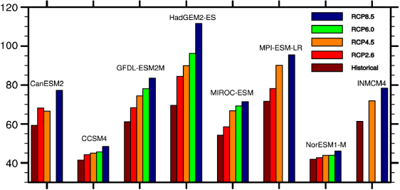
Figure 1. The mean global annual Rh (Pg C) during 1976–2005 from historical simulations using eight ESMs and during 2071–2100 under four different RCPs [25].
Download figure:
Standard image High-resolution image2.3. ESM Rh parameterization
The Rh parameterization as a function of temperature, soil moisture, and other processes is similar across different ESMs; it differs usually in the exact functional forms. The temperature sensitivity in all ESMs except GFDL-ESM2M is represented by the Q10 or Arrhenius equations, both of which are functionally similar. In GFDL-ESM2M, Rh increases with temperature up to an optimal temperature and then decreases. Rh in all of these ESMs either increases monotonically with increasing soil water availability or increases up to an optimal moisture level and then decreases. CCSM4 and NorESM1 include the nitrogen limitation in the Rh computation. The number of litter and soil pools and the temperature and moisture functions are summarized in the table 1 in Todd-Brown et al [26]. For instance, CLM4-CN as used in CCSM4 and NorESM1-M computes Rh through three litter pools, three soil organic matter (SOM) pools, and a coarse woody debris pool as a converging cascade [27]. At each timestep, Rh (g C m−2 s−1) from each pool is calculated as [27, 28]

where k (h−1) is the base pool-specific fixed decomposition rate, C (g C m−2) is the carbon content in the corresponding pool, fr is a fixed fraction of the decomposition carbon flux released as CO2 for specific plant functional type and tissue, fT is based on Q10 of 1.5 averaged over the top five soil layers, and fw is proportional to soil moisture and the weighting depending on soil water potential (averaged over the top five soil layers). The nitrogen limitation fN is computed from the competition between the plant and nitrogen immobilization demand (g N m−2 s−1) for the available soil mineral nitrogen pool. When the available nitrogen pool is insufficient to meet the combined demands, fN is less than 1; otherwise fN is set to 1. For T <− 10 °C or soil water potential <−10 MPa, Rh is taken as zero, consistent with the laboratory measurements [19].
3. Results
3.1. Global patterns of Rh from ESMs and observations
The range of the global Rh estimates from eight ESMs is 41.3–71.6 Pg C a−1 (figure 1), and their average is very close to the empirically inferred values centered around 60 Pg C a−1 [29, 30]. However the two ESMs including coupled carbon–nitrogen dynamics (CCSM4 and NorESM1-M) underestimate the global Rh by 30% compared with these values (figure 1). Compared with the historical period from 1976 to 2005, the global annual Rh from 2071 to 2100 under the RCP2.6, RCP4.5, RCP6.0, and RCP8.5 scenarios is projected to increase by 10.6 ± 6.2%, 17.9 ± 8.6%, 21.8 ± 13.9%, and 31.0 ± 14.9%, respectively, across the eight ESMs, largely due to the increase of global mean surface temperature [31, 32] along with other confounding effects (e.g. increase in vegetation production). In absolute terms this represents widely diverging projected carbon cycle feedbacks in response to environmental change; this was greatest for the RCP8.5 condition (46.0–111.5 Pg C a−1) but the variance is reduced if the two models including a nitrogen cycle are excluded (71.4–111.5 Pg C a−1). The tropical latitudes represent the largest Rh source followed by the boreal latitudes in both historical and 21st century simulations in these eight models. The change of global annual Rh in response to temperature change confounded with CO2 evolution and land use change from 1850 to 2005 varies from −0.56 to +12.6 Pg C °C−1 across the ESMs. In contrast, this rate is just 2.3 Pg C °C−1 in response to temperature change only (18; based on the CASA model with globally variant Q10 values).
Because of the mismatch between point measurements and model grid box output, it is more appropriate to compare the observed and model-simulated ranges of Rh than the direct point-to-point comparisons. There is a substantial overlap between the magnitude of Rh estimated from observations and ESMs across all biomes (figure 2). In temperate forests, agriculture, and grasslands, the median and range of Rh predicted by the two ESMs incorporating the nitrogen cycle (CCSM4 and NorESM1-M) are closest to observed values (figures 2(b), (d) and (e)). In tropical forests, there is little difference between models with and without the nitrogen cycle (figure 2(c)), as the nitrogen supply is sufficient (fN = 1 in equation (1)). Over the boreal forest, however, the constraint of nitrogen results in a significantly lower Rh from CCSM4 and NorESM1-M with the maximum Rh less than 200 g C m−2 (lower than the median rate from observations), while the other six ESMs perform better on average compared with observations (figure 2(a)). Some models without the nitrogen constraint generate Rh values much higher than any observations. For instance, the minimum and maximum Rh values from the six carbon-only ESMs are 135 and 789 g C m−2 over the boreal forest (figure 2(a)), in contrast to 25 and 591 g C m−2 in observations. This deficiency is particularly apparent for temperate ecosystems and tropical forests; the minimum Rh from MPI-ESM-LR is as high as 379 g C m−2, far above the observed minimum at 11 g C m−2 (figures 2(b)–(e)).

Figure 2. Boxplot of annual Rh (g C m−2). The box and whisker bars indicate the full range (thin line) and 25th–75th percentiles (upper and bottom edges of the bar) and median (line in the bar) of Rh for the specific year and location of the measurements. The alphabets on the x-axis denote observations (SRDB-V2, blue), the ESMs with the carbon cycle only (CanESM2, GFDL-ESM2M, HadGEM2-ES, INMCM4, MIROC-ESM, and MPI-ESM-LR, red) and with the carbon–nitrogen cycle (CCSM4 and NorESM1-M, purple). The number of records in the panels is 56, 219, 40, 48, and 37, respectively.
Download figure:
Standard image High-resolution image3.2. Response of Rh to environmental drivers
Rh in ESMs at each time step (usually 10–20 min) is regulated exponentially by temperature and linearly by soil moisture, and in CCSM4 and NorESM1-M limited by the availability of nitrogen (equation (1)). Averaging to longer time-steps (e.g., the annual averages) diffuses these relationships and linkages to other environmental drivers emerge. If the relationship between annual variables emerges from the mathematical structure (equation (1)) of ESMs but are absent in reality, then the mathematical structure is deficient. For example, surface temperature explains between 5% for CanESM2 and 43% for INMCM4 of the variance in annual Rh, while the corresponding value from observations is 16% (table 2). NPP explains between 63% and 97% of the variance in annual Rh, over 90% in five of the eight models, in contrast to the observational value of 23% (table S2 available at stacks.iop.org/ERL/8/034034/mmedia). Annual precipitation is a key driver of Rh in ESMs (0.19 ≤ r2 ≤ 0.76) but much less important in observations (r2 = 0.05, table S2). Similarly, the importance of SOC in the Rh computation is overestimated in ESMs compared with observations (table S2).
Table 2. The statistics of the annual Rh (g C m−2) based on the partial least squares (PLS) regression. (Note: covariates for the prediction of ln(Rh) include the annual mean surface temperature (T, ° C), and the logarithms of annual precipitation (Pr, mm), net primary production (NPP, g C m−2), and soil organic carbon (SOC, g Cm−2). The r2 and RMSE values are the coefficient of determination and root mean square error between Rh and fitted values, respectively.)
| T | T,ln(Pr),ln(NPP),ln(SOC) | |||||
|---|---|---|---|---|---|---|
| r2 | RMSE | Q10 | r2 | RMSE | Q10 | |
| SRDB-V2 | 0.16 | 201 | 1.48 | 0.55 | 142 | 1.83 |
| CanESM2 | 0.05 | 255 | 1.13 | 0.98 | 33 | 1.17 |
| CCSM4 | 0.26 | 237 | 1.89 | 0.84 | 109 | 1.97 |
| GFDL-ESM2M | 0.09 | 291 | 1.32 | 0.87 | 82 | 1.71 |
| HadGEM2-ES | 0.22 | 392 | 1.28 | 0.94 | 70 | 1.10 |
| INMCM4 | 0.43 | 250 | 1.74 | 0.95 | 73 | 1.14 |
| MIROC-ESM | 0.22 | 152 | 1.21 | 0.88 | 33 | 1.02 |
| MPI-ESM-LR | 0.27 | 184 | 1.22 | 0.75 | 79 | 1.08 |
| NorESM1-M | 0.22 | 261 | 1.74 | 0.89 | 93 | 1.62 |
As an example, these relationships are illustrated for CCSM4 and observations in figure 3. The regression slope is much greater in CCSM4 than observed, indicating the greater sensitivity of simulated Rh to Pr, NPP, and SOC. The r2 value in CCSM4 is also much greater than observed. Furthermore, the r2 values between Rh and other plant-related variables (e.g., leaf area index (LAI), total vegetation carbon, standing litter carbon) are much greater in CCSM4 than observed. These results are expected, since there is a close causal relationship between LAI and NPP, and vegetation is the only source of the decomposition pools in ESMs, leading to higher correlations of Rh with NPP and SOC in ESMs. In contrast, available observational data from 57 records in SRDB-V2 indicate that only 42% of total Rh is from litter and the rest originates from the SOC and mineral carbon.

Figure 3. The relationship of annual Rh (g C m−2) with annual precipitation (Pr, mm), net primary productivity (NPP, g C m−2), and soil organic carbon (SOC, kg C m−2) from CCSM4 (left panels) and observations (right panels). The slope, coefficient of determination, and the significance level of the regression with a paired Student's t test are given in each panel.
Download figure:
Standard image High-resolution imageMulticollinearity in the environmental driver is investigated here using partial least squares (PLS) regression (see supplementary text S1 available at stacks.iop.org/ERL/8/034034/mmedia) of Rh against annual mean surface temperature (T, ° C) and the three variable in figure 2: annual precipitation (Pr, mm), NPP (g C m−2), and total SOC (g C m−2). Pooling observations over all sites (figure S1 available at stacks.iop.org/ERL/8/034034/mmedia), the apparent Q10 of Rh is calculated as 1.48 by computing the fold change in Rh with respect to temperature variation across all sites. The corresponding values vary from 1.13 to 1.89 (median =1.30) for the eight ESMs (table 2). When other environmental drivers of Rh are factored out, the apparent Q10 is increased to 1.83 in observations, but its change is ESM-dependent (i.e. it is increased in three ESMs but decreased in the remaining five) (table 1). Conclusions are similar if the other two regression methods are used (table S3 available at stacks.iop.org/ERL/8/034034/mmedia). Even though CCSM4 and NorESM1-M adopt the same land model (CLM4-CN), their Q10 values differ from each other (table 2), and interestingly, they differ from the embedded Q10 value of 1.5 for CLM4-CN at each time step in equation (1).
When all four confounded variables T,ln(Pr),ln(NPP), and ln(SOC) are used for the regression of ln(Rh),r2 between Rh and fitted values increases substantially in both observations and ESMs (table 2). While this regression explains 55% of the variance of Rh in observations, it accounts for 75–98% of the Rh variance in ESMs. The root mean square error (RMSE) is also significantly reduced as the covariate number is increased from one to four, but this decrease is more dramatic in ESMs than in observations (table 2). Similar results are obtained using the other two regression methods (table S3).
3.3. Use of observed Rs in ESM evaluations
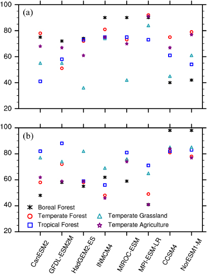
Because observational studies report Rs much more frequently than Rh, we have developed two minimum requirements or 'reality checks' for ESM Rh estimates based on Rs reported in the SRDB-V2 database. While all eight ESMs provide Rh and total respiration (Rh plus plant and root Ra), none of these ESMs provides Rs as a standard output. Since total respiration includes Rs and plant Ra, the first requirement is that total respiration from ESMs should not be less than observed Rs. Similarly, since Rs includes Rh and root Ra, the second requirement is that Rh from ESMs should not be greater than observed Rs. The percentage of sites where the first requirement is met varies from 40% to 90% (figure 4(a)), while it is higher and varies from 41% to 98% for the second requirement (figure 4(b)). The first requirement is met at most sites over the boreal forest in the six carbon-only ESMs, but it is met at just 41% of the sites in the two ESMs with the carbon–nitrogen cycle. In contrast, the second requirement is met at 98% of the sites over the boreal forest in these two ESMs, while the percentage is much lower (41–62%) in the other six ESMs (figure 4(b)).
Figure 4. The percentage of the records (a) where the simulated (heterotrophic and autotrophic) respiration is not less than the soil respiration in SRDB-V2 and (b) where the simulated Rh is not greater than the soil respiration in SRDB-V2.
Download figure:
Standard image High-resolution image
Note that more models (than the eight used in this study) and more ensemble members from each model are also available now from CMIP5 [25], but their Rh treatments are similar to those discussed here. Therefore the above conclusions are expected to be little affected, even though quantitative values (e.g., the exact values in figure 4) would be changed.
4. Discussion
4.1. Spatial scale mismatch and data uncertainty
There is a horizontal scale mismatch between point measurements and model grid box output. There is also a vertical scale mismatch between point measurement of environmental variables (e.g. temperature) and model output based on multiple soil layers. The latter mismatch is less serious for annual (mean or accumulated) variables. For instance, annual mean temperature is relatively close to each other in different soil layers. The Rh data in SRDB-V2 also contain uncertainty due to the use of different methods to partition observed Rs into heterotrophic and autotrophic respirations. Table 1 summarizes these partitioning methods and indicates that the mean Rh:Rs ratio in the SRDB-V2 database varies from 0.45 to 0.65 (and the median ratio varies from 0.44 to 0.70) depending on the method used. These factors are partially responsible for the above model-data inconsistencies, particularly for the direct Rh comparison between observations and model output (figure 2). Their impact on the comparison of the relationship between Rh and other variables (figure 3, tables 2, S2, and S3), however, is expected to be much less. The correlation between annual Rh and Pr, NPP, and SOC and between the logarithm of annual Rh and T are much higher in ESMs than in observations (tables 2 and S2). The annual Rh is also more sensitive to these climatic, vegetation, and edaphic variables in ESMs than in observations, as indicated by the regression slopes in figure 3.
While soil respiration can be observed directly, 'observations' of Rh are derived from a range of methods (table 1). For this reason, there are many more Rs observations than Rh data. Furthermore, both annual and seasonal Rs data are available from SRDB-V2, while seasonal Rh is not available. To make use of Rs observations, we have created two 'reality checks' for ESMs. All models (with or without the nitrogen cycle) fail to pass these tests in all biomes a significant percentage of the time (figure 4). To facilitate more explicit model validation and improvements, modeling groups should provide Rs as a standard output in the future.
4.2. Guidance on Rh improvements in ESMs
The Rh computation in ESMs is dependent on various factors (equation (1)), including the availability of nitrogen [27, 33]. Without the nitrogen constraint, some ESMs tend to produce Rh values much higher than observations (figure 2). The two models that include an explicit nitrogen cycle perform very well in temperate biomes and might be expected to show more realistic mechanistic Rh responses. However, the nitrogen constraint appears to be too severe in the boreal forest (figure 2), which may explain the particularly low global Rh estimates for CCSM4 and NorESM1-M relative to the other models (figure 1). To test the robustness of this conclusion, we have evaluated another ESM incorporating the nitrogen cycle from China (BCC-CSM1.1 [34, 35]) and found that this model compares well with Rh derived from observations. For example, the 25th, 50th (median) and 75th percentiles of annual Rh over the boreal forest are 221, 323 and 341 g C m−2, in good agreement with observations in figure 2(a). Furthermore, the lower Rh than expected over the boreal forest in CCSM4 and NorESM1-M is unlikely to be related to the turnover times for global soil carbon in these two models: the turnover times across the CMIP5 ESMs range from 11 to 39 years, in which CCSM4 (about 12 years) is in the lower end but NorESM1-M is in the middle of the range [26]. These analyses and the high correlation between Rh and NPP (figure 3(c), table S2) suggest that low Rh estimates in both models are most probably caused by low NPP which is associated with high Ra. Therefore, the treatment of Ra in both models needs to be improved, including the maintenance respiration (as a function of temperature and tissue nitrogen concentration) and growth respiration (proportional to the difference between leaf photosynthesis and maintenance respiration).
Change in CO2 release from terrestrial ecosystems is dependent on the temperature sensitivity (Q10) of autotrophs and heterotrophs, which has received much attention in recent years with some controversy [18, 22, 36–38]. However, much less attention has been paid to the use of observed intrinsic and apparent Q10 values in ESMs. The intrinsic (or unconfounded) temperature sensitivity (quantifying the inherent kinetic properties of substrate decomposition) is found to converge to 1.4 ± 0.1 based on flux tower measurements across different biomes [37], and the embedded Q10 value of 1.5 used in the Rh computation at each time step in CLM4-CN (equation (1)) falls into this range. The apparent Q10 is typically calculated from the short-term temporal variability of measured Rh and temperature, and it represents the temperature sensitivity confounded by other factors that covary with temperature. The apparent Q10 values in CCSM4 and NorESM1-M (adopting the same CLM4-CN) differ from each other and from the embedded Q10 value of 1.5. The apparent Q10 values vary broadly from 1.43 to 3.43 in the SRDB-V2 database (figure S1 available at stacks.iop.org/ERL/8/034034/mmedia) and differ from the intrinsic values of 1.4 ± 0.1. In contrast, the apparent Q10 using annual Rh and T across all sites in figure S1 is 1.48, coincidentally close to the embedded value in CLM4-CN and the intrinsic Q10 values from flux tower measurements [37]. The Q10 values are also sensitive to the number of covariates considered in observations and ESMs (tables 2 and S2). For the same climate models, the Q10 values in table 2 are also different from those computed based on the linear regression of ln(SOC) with ln(NPP) and T in the table 4 of Todd-Brown et al [26]. Because Q10 can be, and has been, calculated in a variety of ways, it is crucial to clearly explain methods used to calculate Q10 to avoid confusion between the modeling and measurement communities.
In ESMs, the Rh computation is proportional to the base pool-specific fixed decomposition rate, the carbon content in the corresponding pool, and the fraction of the decomposition carbon flux as CO2 (equation (1)). With such simple treatments, it is not surprising that the annual Rh is much more sensitive to SOC in ESMs than in observations, as indicated by the regression slopes in figures 3(e) and (f). In contrast, there is essentially no statistically significant relationship between SOC and Rh in SRDB-V2 (figure 3(f)) and in an empirical study [10] for several possible reasons. Not all organic compounds are equally accessible to microorganisms [12]. Labile carbon from root exudates and nutrient content in SOC are important in controlling Rh [38, 39]. Rh is differentially controlled within and outside of the rhizosphere and inhibited in low oxygen conditions [15] and is strongly regulated by extracellular microbial enzymes dependent on the dynamics of microbial function, population size and nutrient availability [31, 33, 36, 40–43]. ESMs omit these mechanisms (figure 3(e)) despite including enzyme-driven process in photosynthesis [44]. In some models the problem is more fundamental. For instance, the soil organic matter carbon to nitrogen ratio is nearly constant at 10 in CLM4-CN, whereas the ratio varies in a broad range of 7–26 in different ecosystems in SRDB-V2. To improve the Rh computation, one promising approach is to incorporate a microbial biomass pool and constraints of extracellular enzymes (e.g. [31]) to represent direct coupling between microbes and soil carbon turnover, mimicking the thermal adaptation and acclimation of Rh by predicting the microbial growth efficiency and respiratory capacity [45].
Note that the lack of statistically significant spatial correlation between annual SOC and Rh over various sites in SRDB-V2 is not necessarily counter to the conventional wisdom on the positive temporal correlation between SOC and Rh over a given site; rather a strong linear relationship is not expected [11]. While more observational data are still needed to establish complex and likely non-linear relationships between annual SOC and Rh in contrasting conditions, the simple treatment of the above three factors used in the Rh computation in ESMs needs to be revised. For instance, the constant decomposition rate in equation (1) may be relaxed to be dependent on soil depth, and the simple carbon allocation rule may need to consider ecosystem acclimation and adaptation.
Because Rh parameterizations in current ESMs lack key regulatory processes like the role of different carbon substrates, microbial dynamics and nutrient constraints, the global Rh range is as large as 17.4 Pg C a−1 (=71.6–54.2) from 1976 to 2005 using the six carbon-only ESMs, and it increases to 40.1 Pg C a−1 from 2071 to 2100 under the RCP8.5 scenario. When the two models with the carbon–nitrogen cycle are also included, these ranges become even larger, reaching 30.3 and 65.5 Pg C a−1, respectively. To reduce such large uncertainties in ESM Rh projections, the observational and ESM community need to work together to design field experiments for testing and improving the Rh parameterization as a function of soil temperature, moisture, and other processes (e.g. equation (1)), rather than just the Q10 factor. Seasonal Rh data, which are not available from SRDB-V2 but are very useful for model Rh evaluations, need to be developed and observations of Rh and likely drivers of microbial metabolism in contrasting conditions would be instructive. In addition to comparing measured flux rates to those predicted by models, model development would be aided by benchmarking mean residence times of C pools used by models against estimates from the field or laboratory based on isotopic or incubation experiments.
Acknowledgments
This work was supported by NSF (AGS-0944101), DOE (DE-SC0006693 and DE-ER65088), CAS (XDA05110103) and NSFC (41305096). The authors thank B Bond-Lamberty for making available the comprehensive soil respiration database, and acknowledge the modeling groups from BCC, CCCMA, GFDL, INM, MIROC, MOHC, MPI-M, NCAR, and NCC; and the World Climate Research Program's (WCRP) Working Group on Coupled Modeling (WGCM) for making the model output available on the US Department of Energy PCMDI server.