
Abstract
A consensus regarding the impact of solar variability on cloud cover is far from being reached. Moreover, the impact of cloud cover on climate is among the least understood of all climate components. This motivated us to analyze the persistence of solar signals in cloud cover for the time interval 1984–2009, covering two full solar cycles. A spatial and temporal investigation of the response of low, middle and high cloud data to cosmic ray induced ionization (CRII) and UV irradiance (UVI) is performed in terms of coherence analysis of the two signals. For some key geographical regions the response of clouds to UVI and CRII is persistent over the entire time interval indicating a real link. In other regions, however, the relation is not consistent, being intermittent or out of phase, suggesting that some correlations are spurious. The constant in phase or anti-phase relationship between clouds and solar proxies over some regions, especially for low clouds with UVI and CRII, middle clouds with UVI and high clouds with CRII, definitely requires more study. Our results show that solar signatures in cloud cover persist in some key climate-defining regions for the entire time period and supports the idea that, if existing, solar effects are not visible at the global level and any analysis of solar effects on cloud cover (and, consequently, on climate) should be done at the regional level.
Export citation and abstract BibTeX RIS

Content from this work may be used under the terms of the Creative Commons Attribution-NonCommercial-ShareAlike 3.0 licence. Any further distribution of this work must maintain attribution to the author(s) and the title of the work, journal citation and DOI.
1. Introduction
The topic of possible solar variability effects on cloud cover is under heavy debate, since there is yet no agreement regarding possible long-term relationships between various solar proxies and cloud cover of different types. Dickinson (1975) suggested that cloud cover might be favored by a higher cosmic rays (CR) flux due to cloud condensation nuclei increase in response to the cosmic ray induced ionization effects (Dorman 2004). Some time ago Svensmark and Friis-Christensen (1997) claimed a striking, almost one-to-one correlation between the global cloud cover and solar activity. Later studies showed that the correlation is more likely restricted to low clouds (Marsh and Svensmark 2000), and to latitudinal bands (Usoskin et al 2004). Harrison and Stephenson (2006) have shown that during days with high cosmic ray flux the probability of the sky to be overcast is somewhat higher, implying that low clouds may be responding to CR flux. Sloan and Wolfendale (2008) argued that less than 25% of the cloud variation seemingly associated to CR flux in solar cycle 22 could be attributed to cosmic ray flux variation. The problem of possible cloud masking in satellite data was raised by Pallé (2005) and re-addressed by Usoskin et al (2006), who showed that correlations based on global or latitudinal averages of the cloud cover might be erroneous, thus the most appropriate analysis should be applied to specific geographical areas. This was done by Voiculescu et al (2006, 2007) who also showed that the possible effect of solar activity on clouds is not uniquely described by one solar proxy, and suggested that clouds in different geographical regions and at different heights can be linked to solar activity by different mechanisms. Gray et al (2010) concluded that current data gives no support to a significant relationship between clouds and CR. It is difficult to say whether the sensitivity of cloud occurrence to solar variations is higher in the upper or in the lower troposphere, since theoretical studies (Yu et al 2008, Kazil and Lovejoy 2004) show that the upper tropical troposphere is more favorable to aerosol nucleation, while Yu (2002) found that the conditions in the lower troposphere lead to a larger variation of ionization associated with solar cycle variations. Kristjansson et al (2004) suggested that the positive correlation between cloud cover and CR flux is in fact a result of the negative correlation between cloud cover and Total Solar Irradiance (TSI), which anti-correlates with cosmic rays. Later Erlykin et al (2010) concluded that only correlations between low or middle clouds and solar irradiation could be real, as well as the correlation between low clouds and cosmic rays. Thus cosmic rays and solar radiation might both act on clouds in a complementary way or they might have opposing effects.
In this paper we investigate whether correlations between low, middle and high cloud cover, and two solar proxies, i.e. cosmic ray induced ionization (CRII) and UV irradiation (UVI), are consistent for the entire period for which International Satellite Cloud Climatology Project (ISCCP) cloud data are available, namely 1984 through 2009. Our aim is to investigate further if the correlations found earlier for shorter intervals (e.g., Marsh and Svensmark 2000, Usoskin et al 2004, Kristjansson et al 2004, Voiculescu et al 2006, 2007) remain consistent when a larger time span is considered. We use correlation and wavelet analyses and identify geographic regions where correlations could be real, and then use the results to identify the most probable solar proxy that might be related to clouds in different areas.
2. Data analysis and method
We use here cloud and solar proxy data spanning over 26 years, i.e. on the interval 1984–2009, fully covering solar cycles (SC) 22 and 23. Cloud data are taken from the ISCCP project (Rossow et al 1996) and are separated into low, middle and high clouds, depending on the cloud top pressure P: low (L), middle (M) and high (H) clouds for P > 680 mbar,440 mbar < P < 680 mbar and P < 440 mbar, respectively (Rossow et al 1996). We acknowledge that ISCCP data should be used with care, especially regarding global data, total cloud or latitudinal averages (Pallé 2005, Usoskin et al 2006, Voiculescu et al 2009, Brown 2008, Kristjánsson et al 2008, Gray et al 2010). The cloud amount, given as percentages of the area covered by clouds of a given type, is obtained from monthly values of the cloud coverage for the period 1984–2009 as given by the ISCCP-D2 IR dataset (http://isccp.giss.nasa.gov), in a geographical grid of 5° × 5°. Besides possible satellite observational problems, which may induce some abrupt changes and trends due to modifications in the satellite view angles (Evan et al 2007, Gray et al 2010, Laken et al 2012), one must also take into account that clouds can be affected by internal climatic factors, such as the Northern Atlantic Oscillation (NAO) or the El Niño Southern Oscillation (ENSO) (e.g. Laken and Pallé 2012). Laken and Pallé (2012) compared MODIS and ISCCP total cloud data for 8 years (2000–8) and found that similar changes appear in both ISCCP and MODIS datasets, but they are larger and more statistically significant in ISCCP. They also show that the agreement gets weaker for high latitudes. In order to avoid this, data were detrended by subtracting the best linear least-square fit. The CRII is calculated using the model of Usoskin and Kovaltsov (2006) and Usoskin et al (2010). The global UVI is calculated using NOAA–Mg II wing-to-core ratio data produced by Space Environment Technologies (www.spacewx.com/AboutMgII.html) (Viereck et al 2001) and zenith angles.
Cloud, CRII and UVI data were annually averaged to exclude the seasonal variability, and all time series were detrended, thus 'cloud data', 'UVI', 'CRII' hereafter refer to the detrended annual data. Correlation maps were produced (an example can be seen in figure 1), in a similar manner to our previous works (Voiculescu et al 2006, 2007). Geographical grid cells where the correlation is significant at the 90% or better level are marked in blue (negative) or red (positive) (i.e. correlation coefficients greater then 0.33). Regions where significant correlation appears systematically in more than 8–10 adjoining grid cells (preferably over more than 10° in latitude or longitude) were defined visually and encompassed by numbered rectangular regions. Geographical location and climate characteristics have also been considered when regions were selected. The mean annual cloud amount inside these selected regions was computed, together with the corresponding annual means for CRII and UVI values, and several time series were obtained for each cloud-solar proxy pair and each region.
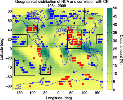
Figure 1. Correlation map between high cloud cover and CRII (negative correlation: blue dots, positive correlation; red dots, 90% confidence) and average high cloud cover for 1984–2009.
Download figure:
Standard imageNext, the coherence and coherence phase between solar proxy and cloud cover was computed using a code developed by Grinsted et al (2004), adjusted for our particular task. The coherence corresponds to the cross-correlation between two time series as a function of frequency and time (e.g. Torrence and Compo 1998) or can be seen as a localized correlation coefficient in time frequency space (Grinsted et al 2004). An example can be seen in figure 2, where the coherence phase is indicated by arrows whose angle is measured relative to the horizontal line (Grinsted et al 2004). Significance of the coherence is tested against red noise, and the 95% confidence level is shown by thick black contours. The coherence power of the two series in selected periodicity bands is shown using color coding, with red showing the highest power at the 95% confidence level (Grinsted et al 2004). The thin black line shows the limit of the cone of influence (COI), which is the region where edge effects become important and the analysis is unreliable (Torrence and Compo 1998). The width of the COI depends on the frequency/period and the lighter tone used in coloring indicates the fact that results in this area should be discarded. Arrows pointing sharp right (left) mean that the two analyzed time series are in phase (anti-phase), while arrows pointing down (up) mean a lag between the two series. A phase angle of −90° (arrow down) could be interpreted as a lag of 2–3 years (i.e. a quarter of the corresponding period) between the solar proxy and cloud series, while a +90° angle (arrow up) would mean a lag of 6–9 years or a lead of 2–3 years. The uncertainties associated with the relative phasing of two noisy signals with common periods were computed as a function of the noise-to-signal ratio. Details are given in the appendix. All wavelet coherence tests were done using the solar proxy as the leading series. Phases are shown only for significant coherences. The frequency band of 9–13 years, considered as representative for the solar cycle, is also shown.

Figure 2. Wavelet coherence between high cloud and CRII for selected regions in figure 1. Continuous black line shows area of 95% confidence and dash black lines indicate the 9–13 years solar cycle periodicity band. Red-to-blue color code is associated with the coherence power between the two series. Arrows indicate the relative phase by their angle relative to the horizontal line. Arrows pointing sharp right (left) mean that the two analyzed time series are in phase (anti-phase), while arrows pointing down (up) mean a lag between solar signal and clouds. See text for details.
Download figure:
Standard imageWe check the relative phase of the solar proxy and clouds, for the frequency band of 9–13 years centered on the solar cycle periods, outside the COI, where edge effects might affect the results (Torrence and Compo 1998). The correlation is considered to be real/consistent if three conditions are met for the 9–13 years band: (1) the coherence is significant outside the cone of influence (i.e. arrows exist outside the cone of influence); (2) the deviation of the relative phase from 0 or π is within the uncertainty limits (i.e. smaller than 30°–45°, see appendix); (3) both previous conditions are met for the entire time interval considered.
3. Results and discussion
First we analyze the relationship between high cloud amount (HCA) and CRII, shown in figure 1. The coherence analysis has been performed for four regions with negative correlation (1–4) and two regions with positive correlation (5 and 6) (figure 2). The correlation appears consistent in all regions where anti-correlation is observed (1–4), with the relative phase being close to π within the phase uncertainties. This is seen in oceanic pristine areas at high northern latitudes and over other limited areas, mainly at northern tropical and southern mid-latitudes of the Pacific Ocean. The response of clouds to CRII seems to come almost instantaneously, considering the phase uncertainty, which is 30°–45°. The negative correlation is better in areas where the cloud amount is small to medium. When the cloud amount is large the correlation seems to decrease, as for instance in the arctic region (4) over Greenland.
The positive CRII–HCA correlation, observed at tropical-temperate latitudes over continental areas Asia (region 5) and in the central Northern America (region 6), is less reliable. The coherence is weak and the relative phase is always greater than 45°, i.e. outside the 1σ uncertainties (figure 2), suggesting that the relation may be spurious. The cloud amount in these regions is relatively small (see figure 1).
Relative phases between solar proxies and clouds which significantly differ from zero (or π for anti-phase relations) can be interpreted as lags or leads, depending on the angle relative to zero. This formally means that, in regions 5 and 6 of figure 1, CRII lags the cloud variations by about 1–2 years, or that cloud leads CRII variation, which makes no sense from the solar-terrestrial point of view. This implies that high cloud variations may be linked to solar radiation, which precedes CR variations by 0–2 years (Usoskin et al 1998). Thus a possibility exists that the positive correlation of HCA with CRII is rather a result of the anti-correlation with UVI. A comparison between the two maps of HCA correlations shows that, indeed, regions 5 and 6 of the HCA–CRII map correspond to regions of opposite correlation of HCA with UVI, i. e. regions 3/4 and 1, respectively, in figure 3.
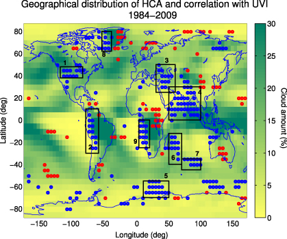
Figure 3. Correlation map between high cloud cover and UVI (negative correlation: blue dots, positive correlation; red dots, 90% confidence) and average high cloud cover for 1984–2009.
Download figure:
Standard imageThe results of the coherence analysis for the correlation between HCA and UV are shown in figure 4. The negative HCA–UVI correlation is consistent only in region 1, over central North America. The relative phase is small and the correlation is significant over the entire interval, suggesting that in this particular region HCA may respond to UVI rather than to CRII variation. For regions 3, 4, 6 and 7 the coherence becomes significant only after 1996, i.e. during SC23, when the two series are in almost exact anti-phase. The phases vary by more than 90°, which suggests that the correlation in this region is due to the strong phase lock of the two series in SC 23. Variations of clouds and UVI in areas 2, 5, 8 and 9 lack any coherence, while over the Indian Ocean and South-West Asia, HCA is connected to UVI only after 1996, i.e. during SC23. In general, except for central northern America, the assessment of the HCA–UVI relationship is problematic.
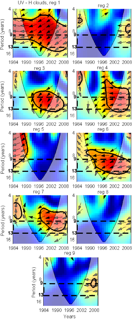
Figure 4. Wavelet coherence between high cloud and UVI for selected regions in figure 3. Continuous black line shows area of 95% confidence and dash black lines indicate the 9–13 years solar cycle periodicity band. Red-to-blue color code is associated with the coherence power between the two series. Arrows indicate the relative phase by their angle relative to the horizontal line. Arrows pointing sharp right (left) mean that the two analyzed time series are in phase (anti-phase), while arrows pointing down (up) mean a lag between solar signal and clouds. See text for details.
Download figure:
Standard imageConcluding, one could say that high clouds over Pacific areas and at high latitudes are likely related to CRII, while small continental areas such as north-west America respond formally better to UVI variations. Central Eurasia and the Indian Ocean are also regions of interest, since correlations with both solar proxies appear, however, during one single cycle, which is not enough for assessing the existence of any relationship.
Five regions of negative correlation (regions 1–5) and one of positive correlation (region 6) between middle cloud amount (MCA) and CRII have been selected in figure 5. The corresponding coherence analysis is shown in figure 6. The coherence is significant and consistent in regions 2 and 3, above large area at northern high latitudes, over Northern Eurasia and neighboring Arctic Ocean and over the extratropical-mid-latitude part of southern America, where the relative phase is close to zero and coherence is strong. In region 4 (northern American high latitudes) coherence exists before 1996, during SC22. On the other side of the Earth, in region 5, i.e. over high latitudes of Indian Ocean, coherence exists only during SC23. In region 1 the correlation lacks power, therefore phase indication is missing. The cloud amount is medium to high everywhere where the correlation is significant.
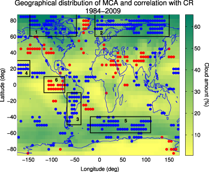
Figure 5. Same as figure 1 but for middle clouds.
Download figure:
Standard image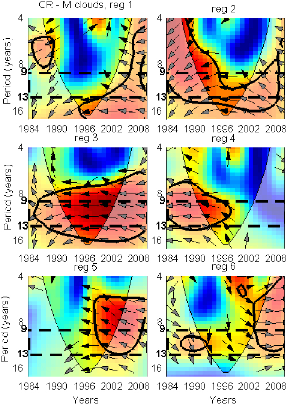
Figure 6. Wavelet coherence between middle cloud and CRII for selected regions in figure 5. See figure 2 for other details.
Download figure:
Standard imagePhases in region 6, west of Peru give no reliable information for assessing the positive correlation. The phase is generally within the uncertainty limit (see the appendix), except the time between 1992 and 1998 (solar min), when the phases vary largely. Also, the coherence is not strong enough outside the cone of influence. Since this is a region vulnerable to El Niño effects, it is difficult to draw any conclusion about the relationship with any of the two solar proxies.
In the MCA–UVI correlation map shown in figure 7, four regions have been selected, two (1 and 2) with negative and two (3 and 4) with positive correlations. In all four regions clouds are almost in phase/anti-phase with the solar trigger, as one can see in figure 8. Although power is not high in some regions (1 and 4), the phase variation is small, around zero, thus one could say that for this case both negative and positive correlations are supported by the coherence analysis. In mid-latitude regions of North America and west off, above the Pacific Ocean, the negative correlation is weaker. However, the correlation is seen during the entire interval and is coherent. The positive relationship is strong above southern Asia and over Siberia and adjacent oceanic regions. Thus the relationship of middle clouds with UVI is better defined than with CRII.

Figure 7. Same as figure 3 but for middle clouds.
Download figure:
Standard image
Figure 8. Wavelet coherence between middle cloud and UVI for selected regions in figure 7. See figure 4 for other details.
Download figure:
Standard imageCorrelations of low cloud amount (LCA) both with UVI and CRII are shown in figures 9 and 11. They are more consistent and extend over larger areas then the other two types of clouds. This was expected from previous results (Usoskin et al 2004, Kristjansson et al 2004, Voiculescu et al 2006, Erlykin et al 2010). The debated positive correlation between low clouds and CRII is seen in regions 1–7 in figure 9 and is supported by the results of the coherence analysis in most regions, shown in figure 10.
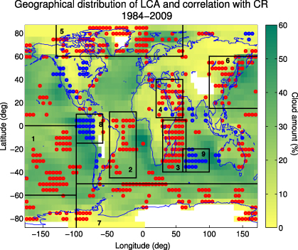
Figure 9. Same as figure 1 but for low clouds.
Download figure:
Standard image
Figure 10. Wavelet coherence between low cloud and CRII for selected regions in figure 9. See figure 2 for other details.
Download figure:
Standard imageThus LCA varies almost in phase with CRII above oceanic areas (southern Atlantic Ocean and western Indian Ocean—regions 2, 3) and in the northern high latitude (region 5). Low clouds over the southern Pacific Ocean and continental East Asia (influenced by the western Pacific) (regions 1, 6) are also almost in phase with CRII, but the relative phase is slightly greater, up to 30°, still within the phase uncertainties. The coherence is less clear in regions 4 and 7; some phase lock exists but it is significant mainly inside the cone of influence. In region 7 low clouds are composed of ice and water, which might respond differently, relative to purely water clouds in low mid-latitudes, to solar forcing. The hemispheric difference in the CRII–LC relationship at high latitudes (good correlation in the north, poor correlation in south) might be due to the fact that clouds are primarily influenced by winds, pressure fields, ocean–land coverage, sea surface temperature (SST), and atmospheric oscillations (e.g. NAO in the north, ENSO in the south) (Chaboureau and Claud 2006, Chiacchio and Wild 2010), which are different between the two hemispheres and which could also respond differently to solar activity (Gabriel et al 2011, Meehl et al 2009, Woollings et al 2010).
Negative LCA–CRII correlation is observed in regions 8 (western coast of South America) and 9 (Indian Ocean), where the coherence is only marginally significant, and phases vary largely to more than 90° (figure 10). The coherence improves during SC23 and the existence of such a perfect phasing, similarly to the previous findings for HCA, might have some physical meaning.
LCA and UVI are globally anti-correlated in regions 1–8, while regions of positive correlation are marked as 9 and 10, as seen in figure 11. Coherence results in figure 12 show that LCA and UVI are almost perfectly in anti-phase in regions 1–6, i.e. in oceanic regions, corresponding coastal regions and arctic latitudes: southern Pacific (region 1), west middle Atlantic and Central America (2), west southern Atlantic (3), western Indian Ocean and coastal regions (5), western North Pacific and coastal regions (6) and the Arctic Ocean (4). The correlation over areas 7 and 8, in the western Pacific (North and South), is less consistent since the coherence is significant only during SC23 and the relative phase is relatively large, between 30° and 75°, which is barely within the uncertainties. In both regions ENSO plays an important role, which may affect the response of clouds to the solar signal.
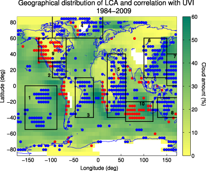
Figure 11. Same as figure 3 but for low clouds.
Download figure:
Standard image
Figure 12. Wavelet coherence between low cloud and UVI for selected regions in figure 11. See figure 4 for other details.
Download figure:
Standard imageThe two regions where LCA correlate positively to UVI are the southern Indian Ocean (region 10) and continental western North America (region 9), but the correlation seems to be good only during SC23. Most of the phases, although formally significant, are unreliable since they are inside the cone of influence, thus none of the positive correlations of LCA to UVI is consistent.
Some of the regions with LCA–UVI correlation correspond to regions in the LCA–CR correlation map. This seemingly makes it difficult to identify the solar proxy responsible for the observed correlation. However, the coherence analysis may help in that, since it allows one to compare relative phases and choose as a favorable proxy the one whose relative phase is closer to zero (somehow similar to the method used in Voiculescu et al (2006), which was based on comparison of correlation coefficients). On the other hand this may be not conclusive when relative phases are small, thus the difference between proxies is not significant. Moreover, a significantly large relative phase (i.e. a phase large enough to be out of the uncertainty interval) may imply a real lag between the solar forcing and the cloud response.
While the mechanism that might connect CRII to cloud cover has been and still is extensively discussed (Harrison and Usoskin 2010, Tinsley and Yu 2004, Gray et al 2010, and references therein) causes of possible connections between clouds and solar radiation are less clear. Whether this is a direct or indirect effect, via other climatic modulation, remains to be seen in subsequent studies. It is presently hardly possible to define a reliable mechanism, due to the large uncertainties related to cloud modeling. We can only speculate here and suggest future possible ways to investigate this relationship. Results shown by, for example, Haigh (2002), Haigh et al (2010), Gray et al (2010), Lockwood et al (2010) and Woollings et al (2010) suggest that the solar UV variability might cause a top-down solar forcing which could lead to regional changes in the tropospheric circulation. This might be transferred to cloud occurrence, formation and characteristics, which could also explain lags that appear in the UVI–LCA relationship. Another possibility is that they relate via SST variations and associated changes in evaporation rates, precipitation and wind systems (Kristjansson et al 2004, Meehl et al 2009), whose response to solar activity is also under debate (Gray et al 2010). Solar modulation of teleconnections (e.g. Dima et al 2005, Bochnícek and Hejda 2005) might also affect cloud occurrence. Recent results show that atmospheric blocking situations, which affect cloud cover (e.g. Chaboureau and Claud 2006), depend on solar activity in the Northern Hemisphere over the Atlantic and Eurasia (Barriopedro et al 2008, Woollings et al 2010). For the Pacific region, Barriopedro et al (2008) have shown that high solar activity induces an enhanced blocking activity in the eastern part, and low solar blocking over the western part. Interestingly, a similar polar behavior over the Pacific is seen also in cloud relationship to UVI: in-phase variation of clouds in the west, anti-phase in the east.
One cannot overlook the fact that in some of the problematic regions (i.e. with incoherent correlation) the coherence appears better after 1996, during SC23. There are important differences between the two cycles SC22 and SC23, since SC23 was much longer and weaker than the previous cycle 22 and it might be possible that high solar radiation has some effect that counteracts the response of clouds to solar proxy. Of course, this could be a simple coincidence and a single cycle is a too small sample to draw any definite conclusion, however some problems that deserve an answer can be raised. In some regions we have found that small relative phases existed outside the areas of significant power, which, according to Grinsted et al (2004), suggests that the link between the two time series might be simply stronger than the one implied by wavelet coherence analysis.
4. Conclusion
We have analyzed the coherence between the time variations of two solar proxy drivers, cosmic ray ionization and UV irradiance, on the one hand, and low, middle and high clouds, on the other hand, in order to check the persistence of solar signal in cloud cover between 1984 and 2009. Coherence plots show that for most of the selected regions cloud type varies in phase or anti-phase with solar activity, depending on cloud type and geographical region. The area where the confidence level is better than 95% is large in many of the coherence plots, which can hardly be a random coincidence.
Based on the fact that significant and consistent correlations were found in some regions, which are different and distributed over the entire globe, we conclude that correlations between cloud cover and solar proxies are real in some key climate defining regions, and investigation of mechanisms relating solar activity variations with cloud cover variations should be continued. On the other hand, the correlation and coherence analysis performed here cannot pinpoint the possible mechanism responsible for such a relation, and a proper model needs to be developed. However, due to the difficulties related to cloud modeling, correlation studies at long and short term scales should also be considered as important, as they can provide empirical evidence suggesting the direction of further research. Obviously the study of cloud response to solar variation cannot rely solely on correlation studies, and studies of cloud microphysics, ion-induced nucleation, effect on various atmospheric circulation pattern on cloud formation or cloud properties are required. Any knowledge, either supporting or contradicting a possible relation between cloud cover and solar activity should help in identifying mechanisms by which clouds could be affected by solar variations.
Acknowledgments
This work was supported by a grant of the Romanian National Authority for Scientific Research, CNCS—UEFISCDI, project number PN-II-ID-PCE-2011-3-0709 (SOLACE). The COST ES1005 TOSCA project is also acknowledged. The ISCCP project is acknowledged for the cloud data. Dave Bouwer and his colleagues from the Space Environment Technologies are acknowledged for the MG II wing-to-core ratio used for our UVI data. Crosswavelet and wavelet coherence software were originally provided by Grinsted.
Appendix:
In order to check the uncertainties of the relative phasing we have performed the following test. Two synthetic purely sinusoidal series with 11 year period were used. A normally distributed noise with the noise-to-signal ratio (NSR—amplitude of the noise relative to the signal) from 0.6 to 3 was added to one wave, keeping the other purely sinusoidal, to reflect the fact that cloud data are noisier than solar proxies. This was repeated 500 times for each NSR, and wavelet coherence analysis was applied, computing the relative phase between the purely sinusoidal and the noisy time series for each of the 500 runs. Finally, the standard deviation of the obtained relative phasing was calculated. The phase difference dependence on the noise amplitude is shown in figure A.1 for 1σ and 2σ levels. Since the two sinusoidal signals are by definition in phase, any deviation from the zero phase in the coherence must come from the noise. The NSR for cloud data was calculated for each cloud series as the ratio between the standard deviation and the amplitude of the 11 year signal found by means of FFT analysis. A typical NSR value for the selected cloud data was found to be 1.5–2. Thus phase differences within ±45° are consistent with zero for these NSR values.
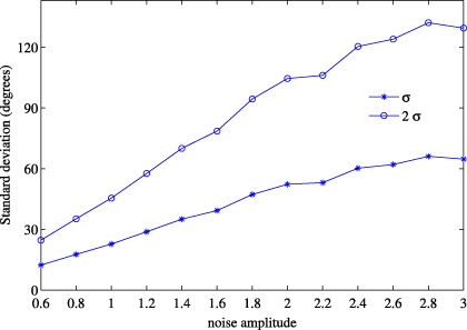
Figure A.1. Uncertainty of relative phasing for different NSR ratio.
Download figure:
Standard image