

Abstract
In coastal habitats artificial structures typically support lower biodiversity and can support greater numbers of non-native and opportunistic species than natural rocky reefs. Eco-engineering experiments are typically trialed to succeed; but arguably as much is learnt from failure than from success. Our goal was to trial a generic, cost effective, eco-engineering technique that could be incorporated into rock armouring anywhere in the world. Artificial rock pools were created from manipulated concrete between boulders on the exposed and sheltered sides of a causeway. Experimental treatments were installed in locations where they were expected to fail and compared to controls installed in locations in which they were expected to succeed. Control pools were created lower on the structure where they were immersed on every tidal cycle; experimental pools were created above mean high water spring tide which were only immersed on spring tides. We hypothesised that lower and exposed pools would support significantly higher taxon and functional diversity than upper and sheltered pools. The concrete pools survived the severe winter storms of 2013/14. After 12 months, non-destructive sampling revealed significantly higher mean taxon and functional richness in lower pools than upper pools on the exposed side only. After 24 months the sheltered pools had become inundated with sediments, thus failing to function as rock pools as intended. Destructive sampling on the exposed side revealed significantly higher mean functional richness in lower than upper pools. However, a surprisingly high number of taxa colonised the upper pools leading to no significant difference in mean taxon richness among shore heights. A high number of rare taxa in the lower pools led to total taxon richness being almost twice that of upper pools. These findings highlight that even when expected to fail concrete pools supported diverse assemblages, thus representing an affordable, replicable means of enhancing biodiversity on a variety of artificial structures.
Export citation and abstract BibTeX RIS

Original content from this work may be used under the terms of the Creative Commons Attribution 3.0 licence. Any further distribution of this work must maintain attribution to the author(s) and the title of the work, journal citation and DOI.
1. Introduction
Urban sprawl—the expansion of humans away from central urban areas on land and its impacts on the environment has long been recognised as a global problem (Van Metre et al 2000, Johnson 2001, Chadwick et al 2006). Recently, 'ocean sprawl'—the proliferation of artificial structures associated with coastal protection, shipping, aquaculture, and other coastal industries (coastal and marine infrastructure (CMI)) is gaining recognition as one of the biggest threats to marine ecosystems (Airoldi and Beck 2007, Firth et al 2013a, Dafforn et al 2015). Globally, coastal development is accelerating with many regions now dominated by artificial coastlines (e.g. Chapman 2003, Lai et al 2015, Burt et al 2013, Firth and Hawkins 2011, Firth et al 2016, Knights et al 2016). Coasts are increasingly 'hardened' as new CMI is proliferating to support and protect burgeoning populations (Thompson et al 2002, Gerland et al 2014). There are however costs associated with replacing natural habitats with hard artificial structures including the loss of ecosystem services provided by those habitats (Beaumont et al 2007, Wyles et al 2014, Knights et al 2015), and alteration of connectivity patterns (Airoldi et al 2015, Bishop et al in press).
Sometimes CMI can provide important ecosystem services such as habitat or protection for species of commercial or conservation importance (e.g. Inger et al 2009, Toft et al 2013, Pearce et al 2014, Firth et al 2015, García-Gómez et al 2015). However, an increasing body of literature described how artificial habitats are poor surrogates for natural rocky reefs; supporting lower biodiversity (Moschella et al 2005, Firth et al 2013b), different communities (Chapman 2003, Evans et al 2016a), and promoting opportunistic and non-native species (Airoldi and Bulleri 2011, Firth et al 2011, Floerl et al 2009, Bracewell et al 2013).
Over 50% of CMI is constructed with Portland cement (Sharma 2009), which, despite being known to be toxic to some marine life (Nandakumar et al 2003, Togero 2006), can support diverse communities (e.g. Griffin et al 2010, Noël et al 2010). Colonising organisms with calcareous skeletons (e.g. oysters, corals) deposit calcium carbonate onto surfaces in a process termed biogenic build-up; which can contribute to the strength and durability of structures (Risinger 2012).
In response to mitigating the potential negative impacts of CMI, the field of eco-engineering has blossomed recently with a particular focus on demonstrating how CMI can be modified to enhance the habitat and promote biodiversity (reviewed in Dyson and Yocum 2015, Dafforn et al 2015, Firth et al 2016), in part, off-setting the negative consequences of lost natural habitat. Techniques include retrofitting novel microhabitats, such as rock pools, pits and surface roughness (Chapman and Blockley 2009, Martins et al 2010, Browne and Chapman 2014, Coombes et al 2015, Evans et al 2016a), deployment of precast concrete units (Perkol-Finkel and Sella 2014, 2015, Firth et al 2014a, Sella and Perkol-Finkel 2015, Loke and Todd 2016) and the transplantation of habitat-forming species onto artificial structures (Perkol-Finkel et al 2012, Ng et al 2015, Ferrario et al 2016).
The majority of eco-engineering experiments has been implemented at small spatial scales, with poor replication, limited monitoring and understandingly, designed to succeed. Thanks to the recent surge of research in this area coastal managers are now faced with a toolkit of potential mitigation and reconciliation options when planning coastal infrastructure (see Dafforn et al 2015, Firth et al 2016 for reviews). However, all too often decisions about 'ticking the green box' are made without consulting ecologists and thus projects can potentially fail, wasting taxpayer's money. Perhaps even more serious is the possibility that the promise of incorporating eco-engineering into development plans may be used as a ploy for getting the green light on harmful coastal developments. Arguably, it is more important to know when schemes fail than when they succeed, as greater knowledge is gained from failure than from success.
To date, eco-engineering experiments conducted in the intertidal zone are largely carried out below mean high water spring tide (MHWS) where biodiversity enhancement is likely to be most successful due to more favourable abiotic conditions lower on the shore (Raffaelli and Hawkins 1996, Firth et al 2013b). Furthermore, trials are typically carried out under particular wave exposure conditions (e.g. Browne and Chapman 2011, Firth et al 2014a, Evans et al 2016a) making it difficult to generalise about success outside of the environmental conditions experienced at that location. The primary aim of our study was to trial a novel eco-engineering technique under conditions in which it was expected to succeed and compare the outcomes to treatments installed in conditions where it was expected to fail. The objective was two-fold. Firstly, to demonstrate proof-of-concept of a new technique, but secondly and perhaps more importantly, to identify where such an approach may not be suitable, thereby minimising the likelihood of investment in unsuitable technology and preserving consumer confidence (e.g. Knights et al 2014) in reconciliation and conservation efforts.
Artificial rock pools were created from concrete manipulated between boulders beneath the precast concrete hollow-core Shepherd Hill energy dissipation (SHED) units on a causeway in Galway Bay, Ireland (figure 1). The causeway offered a unique opportunity to trial the same technique under different environmental conditions simultaneously within a small spatial area. The west side of the causeway is exposed to swells coming in from the Atlantic Ocean, whilst the eastern side is relatively sheltered in comparison. Biodiversity patterns differ with varying levels of wave exposure (Ballantine 1961) with sheltered pools typically supporting lower biodiversity than moderately exposed rock pools (Firth, pers. obs.). The SHED units on the causeway were arranged in straight horizontal lines at different shore heights. Previous studies have found an inverse relationship between biodiversity and shore height in artificial habitats (Firth et al 2013b, Browne and Chapman 2014), but no studies to date have investigated the combined effects of wave exposure and shore height on colonisation of eco-engineered habitats.
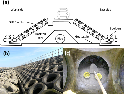
Figure 1. Mutton Island Causeway, Galway Bay, Ireland. (a) Schematic showing engineering design (redrawn form Edger and Murdock 2003); upper Shepherd Hill energy dissipation (SHED) units are positioned 0.4 m above MHWS (4.3 m above Chart Datum); lower SHED units are positioned 1.9 m below MHWS (2.0 m above Chart Datum); (b) image showing the rock armour toe and precast concrete Shepherd Hill energy dissipation (SHED) units on exposed side (Photo: L. Firth); (c) image showing the construction of artificial rock pools at the base of SHED units using quick-drying concrete and buckets (Photo: L. Firth).
Download figure:
Standard image High-resolution imageThe design of the causeway enabled the testing of the efficacy of the artificial rock pools among two different wave exposures ('exposed' and 'sheltered') and two different shore heights ('lower' and 'upper') simultaneously. Reference (control) pools were installed lower on the structure where they were immersed on every tidal cycle and experimental pools installed above MHWS, which were only immersed on spring tides. Upper pools were deliberately placed above MHWS with an expectation of failure (i.e. very few species were expected to colonise the upper pools). We tested two hypotheses: (1) lower pools would support greater taxon and functional richness and different taxon and functional composition than upper pools; (2) exposed pools would support greater taxon and functional richness and different taxon and functional composition than sheltered pools.
2. Materials and methods
2.1. Study area
Galway Bay is a large marine-dominated bay on the west coast of Ireland. The total length of coastline in Galway Bay from Cloghmore, Co. Galway (53°13'N, 9°31'W) to Black Head, Co. Clare (53°09'N, 9°15'W) is 191 km, comprising ∼180 km (93%) natural and ∼12.6 km (7%) artificial coastline. The present length of coastline within the Galway City limits is ∼23 km, comprising ∼13 km (55%) natural and ∼10.5 km (45%) artificial coastline. There are plans to expand the existing harbour to create commercial quays and a deep water docking facility (figure 2); the proposed development will increase the extent of the artificial coastline from 10.5 to 14.6 km (53%), an increase of 39%.

Figure 2. Map showing the extent of existing artificial coastline within the Galway City limits in Galway Bay, Ireland in 2015 (estimated from GoogleEarth). The proposed dock extension is highlighted in grey to the east of the experimental site on the Mutton Island Causeway.
Download figure:
Standard image High-resolution image2.2. Experimental set up
2.2.1. Causeway engineering details
Mutton Island is connected to Galway City by a 0.8 km causeway (figure 2, 53°15'27''N, 09°03'18'' W). The top of the causeway is 1.4 m above MHWS. Precast concrete toe units hold concrete SHED units in place, which are fronted with rock armour toes (figure 1).
In June 2013, artificial rock pools were created by pouring quick-drying concrete around buckets in the base of the SHED units (figure 1(c)). The concrete was sufficiently coarse and dry enough not to run among the boulders beneath, but could be easily manipulated to fill the interstitial spaces among boulders. Once the concrete had set, the buckets were removed to reveal water-retaining depressions (hereafter referred to as a 'pool') of opening diameter 13–14 cm, bottom diameter 10.6 cm and 10–12 cm depth (∼1250 cm3 volume). In total, 80 pools were created: 20 upper (0.4 m above MHWS) and 20 lower (1.9 m below MHWS), and replicated on both the eastern (hereafter 'sheltered') and western (hereafter 'exposed') sides of the causeway.
2.2.2. Sampling
After 12 months (May 2014), all colonising organisms were sampled visually in situ using non-destructive techniques. After 24 months (May 2015), all colonising organisms were removed from the pools and identified to the lowest possible taxonomic level in the laboratory. Flora and fauna were grouped into functional groups based on morphological features (Eriksson et al 2002) and feeding strategies respectively.
2.3. Statistical analyses
To address hypothesis 1—that lower pools would support greater taxon and functional richness and different taxon and functional composition than upper pools, data were treated separately for the 12 month and 24 month sampling periods. To address hypothesis 2—that exposed pools would support greater taxon and functional richness and different taxon and functional composition than pools on the sheltered side, only the data collected after 12 months was used as pools on the sheltered side became inundated with sediment some time between 12 and 24 months and were therefore omitted from analyses.
Analysis of variance (ANOVA) and permutational analysis of variance (PERMANOVA, Anderson 2001) were used to test hypotheses 1 and 2. ANOVA was used to test for differences in mean taxon and functional richness based on presence/absence data. PERMANOVA was used to test for differences in multivariate taxon and functional composition, based on 9999 unrestricted permutations of raw presence/absence data. Percentage contributions of individual taxa and functional groups to dissimilarity between communities were calculated using SIMPER (Clarke 1993). SIMPER analysis in the PRIMER package was used to assess which species were most influential in causing similarity among plots within treatments and dissimilarity among different treatments (Clarke and Warwick 1994). In all cases, the same design was used for ANOVA and PERMANOVA, but with separate designs for 12 and 24 month comparisons. For 12 months, a two-way crossed design was used, with fixed factors Exposure and Shore Height. The 24 month data were analysed using a one-way design with fixed factor Shore Height.
Using 24 month data, the likelihood of species occurring in pools at different shore heights (probability of occurrence) was estimated from incidence matrices (i.e. data describing the presence or absence of a species in a pool, (Dorazio et al 2011)). The sum presence of a species over the number of pools sampled is used to calculate the likelihood of occurrence of a species. This uses binary presence–absence data and not abundance data. Random resampling with replacement was used to generate species accumulation curves to estimate the predicted number of taxa with an increasing number of pools.
Beta diversity which has been defined as the ratio between gamma (regional) and alpha (local) diversities (Whittaker 1960) can also be used as a measure of community heterogeneity (Tuomisto 2010a, 2010b). Here, we used the Sørensen index of dissimilarity (Whittaker 1960) to compare communities in terms of the number of shared and unique taxa recorded in different pools within shore heights. Larger values of beta diversity (i.e. those that tend toward 1) indicate greater dissimilarity between pools. Species occurrence probabilities, species accumulation curves and Sørensen index estimates were calculated using the R package 'Vegan' (Oksanen et al 2016). Pairwise comparisons of beta diversity between pool pairs after 24 months are shown using correlation plots, and non-metric multidimensional scaling used to show dissimilarity in taxon and functional compositions between exposure and shore heights after 12 and 24 month periods respectively.
3. Results
3.1. Biotic colonisation of concrete pools after 12 months
Non-destructive sampling identified 19 taxa from 8 functional groups (table 1(a)). All 19 taxa were recorded in exposed pools in comparison to only 4 in sheltered pools. A greater number of taxa were found in the lower (15) than upper pools (10) on the exposed side.
Table 1. Summary of the number of taxa in each functional group (a) after 12 months and (b) after 24 months in lower and upper pools on exposed and sheltered sides of the Mutton Island causeway, Galway Bay, Ireland.
| (a) 12 months | (b) 24 months | |||||||||
|---|---|---|---|---|---|---|---|---|---|---|
| Causeway | Exposed only | Sheltered only | Exposed | |||||||
| Functional group | Total | Total | Lower | Upper | Total | Lower | Upper | Total | Lower | Upper |
| Thin filamentous | 3 | 3 | 2 | 3 | 1 | 1 | 1 | 14 | 10 | 11 |
| Corticated foliose | 1 | 1 | 1 | 1 | 0 | 0 | 0 | 6 | 4 | 5 |
| Corticated macrophyte | 2 | 2 | 2 | 0 | 0 | 0 | 0 | 4 | 3 | 2 |
| Leathery macroalgae | 0 | 0 | 0 | 0 | 0 | 0 | 0 | 4 | 4 | 2 |
| Calcareous algae | 1 | 1 | 1 | 0 | 0 | 0 | 0 | 2 | 2 | 1 |
| Suspension feeder | 6 | 6 | 5 | 2 | 0 | 0 | 0 | 15 | 15 | 5 |
| Grazer | 3 | 3 | 1 | 3 | 1 | 0 | 1 | 10 | 9 | 5 |
| Detritivore | 1 | 1 | 1 | 1 | 1 | 0 | 1 | 5 | 5 | 3 |
| Carnivore | 0 | 0 | 0 | 0 | 0 | 0 | 0 | 3 | 3 | 0 |
| Omnivore | 2 | 2 | 2 | 0 | 1 | 1 | 0 | 5 | 5 | 2 |
| Other | 0 | 0 | 0 | 0 | 0 | 0 | 0 | 4 | 4 | 1 |
| Total taxon richness | 19 | 19 | 15 | 10 | 4 | 2 | 3 | 72 | 63 | 37 |
| Total functional richness | 8 | 8 | 8 | 5 | 4 | 2 | 3 | 11 | 11 | 10 |
| Unique taxon richness | 35 | 9 | ||||||||
| Rare taxon richness | 13 | 2 | ||||||||
3.1.1. Taxon and functional richness
There was a significant interaction between exposure and shore height for both taxon and functional richness (table 2(a), figure 3(a)). On the exposed side lower pools supported significantly greater mean taxon (4.6) and functional richness (3.6) than upper pools (3.7 and 2.3 respectively), whilst on the sheltered side there was no significant difference between lower and upper pools (figure 3(a)) in either taxon or functional richness.
Table 2. (a) ANOVA comparing taxon and functional richness and (b) PERMANOVA comparing taxonomic and functional composition among exposures and shore heights after 12 months. (c) ANOVA of taxon and functional richness; (d) PERMANOVA comparing taxonomic and functional composition among shore heights after 24 months. Where Cochran's C was significant α was set to 0.01 (Underwood 1997). Significant P-values are in bold.
| (a) 12 months: univariate ANOVA of richness | |||||||
|---|---|---|---|---|---|---|---|
| Taxon | Functional | ||||||
| Source | df | MS | F | P | MS | F | P |
| Exposure | 1 | 33.5868 | 415.9 | 0 | 63.0125 | 81.65 | 0 |
| Shore height | 1 | 0.0937 | 1.16 | 0.2848 | 5.5125 | 7.14 | 0.0092 |
| Exposure X shore height | 1 | 0.3796 | 4.7 | 0.0033 | 7.8125 | 10.12 | 0.0021 |
| Residual | 76 | 0.0808 | 0.7717 | ||||
| Total | 79 | ||||||
| Transformation | Ln(X) | None | |||||
| Cochran's C | NS | P < 0.01 | |||||
| (b) 12 months: multivariate PERMANOVA of community composition | |||||||
| Taxon | Functional | ||||||
| Source | df | MS | F | P | MS | F | P |
| Exposure | 1 | 49 779 | 49.661 | <0.0001 | 44 404 | 79.35 | <0.0001 |
| Shore height | 1 | 11 624 | 11.597 | <0.0001 | 6769.6 | 12.097 | <0.0001 |
| Exposure X shore height | 1 | 16 783 | 16.744 | <0.0001 | 8443.6 | 15.089 | <0.0001 |
| Residual | 76 | 1002.4 | 559.61 | ||||
| Total | 79 | ||||||
| Transformation | SQRT | SQRT | |||||
| (c) 24 months: univariate ANOVA of richness | |||||||
| Taxon | Functional | ||||||
| Source | df | MS | F | P | MS | F | P |
| Shore height | 1 | 90 | 4.55 | 0.0394 | 18.225 | 8.33 | 0.0064 |
| Residual | 38 | 19.7789 | 2.1882 | ||||
| Total | 39 | ||||||
| Transformation | None | None | |||||
| Cochran's C | P < 0.01 | NS | |||||
| (d) 24 months: multivariate PERMANOVA of community composition | |||||||
| Taxon | Functional | ||||||
| Source | df | MS | F | P | MS | F | P |
| Shore height | 1 | 18 551 | 15.6 | <0.0001 | 3534.2 | 10.593 | <0.0001 |
| Residual | 38 | 1189.2 | 333.64 | ||||
| Total | 39 | ||||||
| Transformation | SQRT | SQRT | |||||

Figure 3. (a) 12 months: comparison of mean taxon and functional richness in lower (black bars) and upper pools (grey bars) on exposed and sheltered sides (non-destructive sampling, n = 20, ±SE); (b) 24 months: comparison of mean taxon and functional richness in lower (black bars) and upper pools (grey bars) on exposed side only (destructive sampling, n = 20, ±SE); (c) predicted total species richness (mean ±95% CI) with increasing numbers of pool units in the low shore (black) and upper shore (grey); (d) total number of taxa unique to lower pools (black), unique to upper pools (grey) and shared (white); (e) proportion of taxa that are unique to lower pools (black) and upper pools (grey), actual numbers given and numbers in brackets refer to number of taxa that were observed in a single pool in either lower or upper. Taxa were defined as rare when they occurred in a single pool. (ns = not significant; *P < 0.05;** P < 0.01.)
Download figure:
Standard image High-resolution imageTable 3. Estimated probabilities of occurrence (with 95% confidence intervals) for intertidal marine species occurring in low shore and high pools. Probabilities are estimated at the average value. Shading indicates species not recorded at shore height.
| Lower site occurrence probability | Upper site occurrence probability | |||||||
|---|---|---|---|---|---|---|---|---|
| Species | Median | 2.5% | 97.5% | Rank | Median | 2.5% | 97.5% | Rank |
| Actinia equina | 0.124 | 0.118 | 0.194 | 31 | 0.000 | 0.000 | 0.000 | — |
| Actinia fragacea | 0.049 | 0.045 | 0.065 | 54 | 0.000 | 0.000 | 0.000 | — |
| Amathia sp. | 0.449 | 0.422 | 0.513 | 17 | 0.000 | 0.000 | 0.000 | — |
| Amphipod indet | 0.197 | 0.190 | 0.248 | 27 | 0.099 | 0.097 | 0.138 | 26 |
| Anurida maritima | 0.773 | 0.673 | 0.778 | 9 | 0.646 | 0.610 | 0.666 | 11 |
| Apherusa jurinei | 0.039 | 0.028 | 0.071 | 60 | 0.238 | 0.231 | 0.304 | 19 |
| Aquatic larvae (Chironomidae) | 0.017 | 0.009 | 0.058 | 63 | 0.058 | 0.054 | 0.088 | 32 |
| Austrominius modestus | 0.670 | 0.589 | 0.682 | 12 | 0.040 | 0.035 | 0.061 | 36 |
| Bryopsis sp. | 0.220 | 0.217 | 0.285 | 24 | 0.000 | 0.000 | 0.000 | — |
| Bryozoan indet | 0.086 | 0.074 | 0.146 | 41 | 0.125 | 0.119 | 0.165 | 23 |
| Calliostoma occidentale | 0.063 | 0.054 | 0.107 | 47 | 0.000 | 0.000 | 0.000 | — |
| Callithamnion corymbosum | 0.780 | 0.701 | 0.782 | 8 | 0.232 | 0.228 | 0.276 | 20 |
| Carcinus maenas | 0.706 | 0.616 | 0.708 | 11 | 0.589 | 0.554 | 0.601 | 14 |
| Ceramium sp. | 0.501 | 0.460 | 0.584 | 16 | 0.000 | 0.000 | 0.000 | — |
| Ceramium strictum | 0.000 | 0.000 | 0.000 | — | 0.115 | 0.109 | 0.157 | 25 |
| Chaetomorpha linium | 0.823 | 0.692 | 0.813 | 6 | 0.713 | 0.674 | 0.723 | 8 |
| Chaetomorpha rupestris | 0.000 | 0.000 | 0.000 | — | 0.084 | 0.078 | 0.116 | 28 |
| Chondria dasyphylla | 0.093 | 0.087 | 0.143 | 39 | 0.000 | 0.000 | 0.000 | — |
| Chondrus crispus | 0.932 | 0.875 | 0.940 | 2 | 0.045 | 0.036 | 0.065 | 34 |
| Chordaria flagelliformis | 0.000 | 0.000 | 0.000 | — | 0.254 | 0.242 | 0.311 | 18 |
| Cirriformia tentaculata | 0.114 | 0.099 | 0.160 | 33 | 0.000 | 0.000 | 0.000 | — |
| Cladophora rupestris | 0.833 | 0.753 | 0.844 | 4 | 0.640 | 0.590 | 0.662 | 13 |
| Cladophora sp. | 0.074 | 0.064 | 0.121 | 44 | 0.084 | 0.074 | 0.133 | 29 |
| Colpomenia peregrina | 0.000 | 0.000 | 0.000 | — | 0.086 | 0.081 | 0.115 | 27 |
| Corralina officinalis | 0.288 | 0.278 | 0.344 | 20 | 0.000 | 0.000 | 0.000 | — |
| Coryne pusilla | 0.243 | 0.236 | 0.317 | 23 | 0.000 | 0.000 | 0.000 | — |
| Echinogammarus stoerensis | 0.092 | 0.082 | 0.134 | 40 | 0.000 | 0.000 | 0.000 | — |
| Ectocarpus sp. | 0.941 | 0.905 | 0.943 | 1 | 0.874 | 0.838 | 0.881 | 5 |
| Electra pilosa | 0.039 | 0.028 | 0.071 | 60 | 0.000 | 0.000 | 0.000 | — |
| Eusyllis blomstrandi | 0.120 | 0.113 | 0.158 | 32 | 0.000 | 0.000 | 0.000 | — |
| Fabricia stellaris | 0.162 | 0.152 | 0.210 | 29 | 0.000 | 0.000 | 0.000 | — |
| Flustrellidra hispida | 0.086 | 0.074 | 0.146 | 41 | 0.000 | 0.000 | 0.000 | — |
| Fucus serratus | 0.095 | 0.087 | 0.157 | 38 | 0.000 | 0.000 | 0.000 | — |
| Fucus sp. | 0.133 | 0.128 | 0.222 | 30 | 0.962 | 0.947 | 0.965 | 1 |
| Fucus vesiculosus | 0.055 | 0.044 | 0.089 | 51 | 0.000 | 0.000 | 0.000 | — |
| Gibbula umbilicalis | 0.060 | 0.052 | 0.086 | 48 | 0.000 | 0.000 | 0.000 | — |
| Harmothoe imbricata | 0.162 | 0.149 | 0.218 | 28 | 0.000 | 0.000 | 0.000 | — |
| Jaera albifrons | 0.057 | 0.051 | 0.114 | 50 | 0.000 | 0.000 | 0.000 | — |
| Laminaria sp. juv | 0.870 | 0.816 | 0.880 | 3 | 0.201 | 0.196 | 0.257 | 21 |
| Laomedea flexuosa | 0.274 | 0.260 | 0.347 | 21 | 0.000 | 0.000 | 0.000 | — |
| Lepidochitona cinereus | 0.000 | 0.000 | 0.000 | — | 0.022 | 0.015 | 0.056 | 37 |
| Lipophrys pholis | 0.024 | 0.014 | 0.048 | 62 | 0.000 | 0.000 | 0.000 | — |
| Lithothamnion | 0.660 | 0.558 | 0.673 | 13 | 0.490 | 0.466 | 0.526 | 15 |
| Littorina littorea | 0.215 | 0.208 | 0.289 | 25 | 0.142 | 0.137 | 0.187 | 22 |
| Littorina obtusata | 0.098 | 0.100 | 0.176 | 37 | 0.077 | 0.074 | 0.109 | 30 |
| Littorina saxatilis | 0.253 | 0.247 | 0.328 | 22 | 0.701 | 0.642 | 0.713 | 9 |
| Lomentaria articulata | 0.060 | 0.052 | 0.086 | 48 | 0.000 | 0.000 | 0.000 | — |
| Modiolus modiolus | 0.049 | 0.040 | 0.081 | 55 | 0.000 | 0.000 | 0.000 | — |
| Myriogramme sp. | 0.054 | 0.045 | 0.074 | 53 | 0.000 | 0.000 | 0.000 | — |
| Mytilus edulus | 0.718 | 0.640 | 0.737 | 10 | 0.896 | 0.875 | 0.900 | 3 |
| Nucella lapillus eggs | 0.107 | 0.090 | 0.142 | 35 | 0.000 | 0.000 | 0.000 | — |
| Palaemon serratus | 0.304 | 0.304 | 0.391 | 19 | 0.000 | 0.000 | 0.000 | — |
| Palmaria palmata | 0.042 | 0.035 | 0.073 | 59 | 0.122 | 0.119 | 0.171 | 24 |
| Pandalus montagui | 0.049 | 0.040 | 0.081 | 55 | 0.000 | 0.000 | 0.000 | — |
| Peringia ulvae | 0.055 | 0.044 | 0.089 | 51 | 0.000 | 0.000 | 0.000 | — |
| Plagiostomum vittatum | 0.396 | 0.366 | 0.463 | 18 | 0.043 | 0.037 | 0.063 | 35 |
| Polydora limicola | 0.065 | 0.059 | 0.086 | 45 | 0.000 | 0.000 | 0.000 | — |
| Polysiphonia sp. | 0.823 | 0.733 | 0.826 | 5 | 0.690 | 0.621 | 0.696 | 10 |
| Polysiphonia sp. B | 0.113 | 0.096 | 0.140 | 34 | 0.058 | 0.054 | 0.088 | 32 |
| Procerodes littoralis | 0.083 | 0.080 | 0.128 | 43 | 0.000 | 0.000 | 0.000 | — |
| Red filamentous | 0.000 | 0.000 | 0.000 | — | 0.291 | 0.283 | 0.337 | 17 |
| Rhizoclonium riparium | 0.000 | 0.000 | 0.000 | — | 0.888 | 0.854 | 0.896 | 4 |
| Rhodothaminiella floridula | 0.046 | 0.041 | 0.068 | 57 | 0.000 | 0.000 | 0.000 | — |
| Rissoella opalina | 0.064 | 0.058 | 0.120 | 46 | 0.000 | 0.000 | 0.000 | — |
| Securiflustra securifrons | 0.203 | 0.195 | 0.267 | 26 | 0.000 | 0.000 | 0.000 | — |
| Spirobranchus triqueter | 0.571 | 0.507 | 0.617 | 15 | 0.340 | 0.334 | 0.399 | 16 |
| Spirorbis sp. | 0.821 | 0.740 | 0.824 | 7 | 0.644 | 0.598 | 0.652 | 12 |
| Talitrus saltator | 0.044 | 0.034 | 0.108 | 58 | 0.000 | 0.000 | 0.000 | — |
| Testudinalia testudinalis | 0.000 | 0.000 | 0.000 | — | 0.060 | 0.054 | 0.081 | 31 |
| Ulva intestinalis | 0.105 | 0.097 | 0.154 | 36 | 0.856 | 0.802 | 0.860 | 6 |
| Ulva lactuca | 0.606 | 0.525 | 0.624 | 14 | 0.915 | 0.897 | 0.922 | 2 |
| Ulva linza | 0.000 | 0.000 | 0.000 | — | 0.837 | 0.805 | 0.848 | 7 |
3.1.2. Taxon and functional composition
There was a significant interaction between exposure and shore height for both taxon and functional compositions (table 2(b)). Post hoc pairwise tests revealed significant differences in taxon and community composition (table 2(b), figures 4(a) and (b)) between exposures for both lower and upper pools. Similarly, pairwise tests revealed significant differences in taxon and functional composition between shore heights for exposed but not for sheltered pools (figures 4(a) and (b)). It is clear that there was little variance in the taxon and functional composition in sheltered pools (figures 4(a) and (b)), but far more variance in exposed pools (figures 4(a) and (b)). As predicted, SIMPER analysis revealed that there were greater numbers of taxa and functional groups associated with lower than upper pools and exposed than sheltered pools (table S1). The most diverse habitat was lower exposed pools.
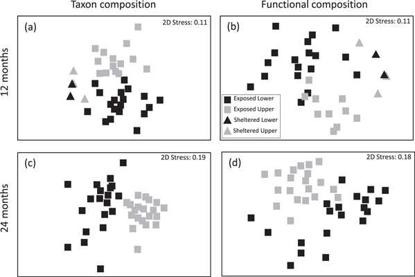
Figure 4. MDS plots of taxon (a), (c) and functional composition (b), (d) compared among the lower (black shapes) and upper pools (grey shapes) on exposed (squares) and sheltered (triangles) sides after 12 months (a), (b); non-destructive sampling, (n = 20) and 24 months (c), (d); destructive sampling, (n = 20).
Download figure:
Standard image High-resolution image3.2. Biotic colonisation of concrete pools after 24 months
Following the 12 month sampling, the sheltered pools became inundated with sediments. Consequently, we refer only to the exposed pools here. After 24 months, destructive sampling yielded 72 taxa across 11 functional groups (table 1(b)). 63 taxa were found in lower and 37 in upper pools (figure 3(c)), two of which classified as non-native: the algae Colpomenia peregrina and the barnacle, Austrominius modestus. Of the 72 taxa recorded, 35 (48.6%) and 9 (12.5%) were unique to the lower and upper pools respectively (table 1, figures 3(d) and (e)).
3.2.1. Taxon and functional richness
There was no significant difference in mean taxon richness between lower (16.9) and upper pools (13.9) (table 2(c), figure 3(b)); but lower pools did support significantly greater mean functional richness than upper pools (8.5 versus 6.7, table 2(c), figure 3(b)).
The community composition in lower pools was more variable than in upper pools (figures 4(c) and (d)), although this variation is largely attributed to a large number of taxa with relatively low probabilities of occurrence (table 3, figure 5; species ranks 38–63). The species with a higher probability of occurrence (>55%) tended to occur in both lower and upper pools (with the exception of Rhizoclonium riparium and Ulva linza). For species less likely to occur (<55% probability of occurrence), 30% were unique to upper and 67% were unique to lower pools.

Figure 5. Probability of occurrence of species (mean ± SD) in lower pools (triangles) and upper pools (circles) (n = 20). The probabilities for individual species and their ranking are shown in table S2. Colours: blue (occur in upper and lower shore heights); orange (unique to low shore); green (unique to upper shore).
Download figure:
Standard image High-resolution imageUnsurprisingly, mean beta diversity of the upper pools (0.39) was lower than that of the lower pools (0.54). Pairwise comparisons of beta diversity between individual pools revealed considerable differences in community composition, even between lower pools established in the same SHED unit (figure 6; L8A versus L8B—β = 0.69), whereas upper pools were more similar (figure 6).

Figure 6. Correlation plots of beta diversity between pools within lower (left) and upper (right) shore heights. Colour bar indicates Sørensen's index of dissimilarity between pool pairs where values nearest to 1 indicate greatest dissimilarity.
Download figure:
Standard image High-resolution image
Comparing taxon accumulation across pools, the number of taxa in upper pools approached asymptote with the inclusion of 11 pools (32 taxa), with only an additional five taxa accumulating across the remaining nine pools (20 pools: 37 taxa). Conversely, for lower pools, the number of species did not reach asymptote (20 pools: 63 taxa; figure 3(c)) with new taxa recorded in nearly every additional pool.
3.2.2. Taxon and functional composition
Composition differed among shore heights for both taxon and functional groups (figures 4(c) and (d)). Of the top ten taxa contributing most to the dissimilarities, five were positively associated with lower and five were positively associated with upper pools (table S3). Of the functional groups that contributed most to the dissimilarities, all but one (corticated foliose) were positively associated with lower pools.
4. Discussion
In this experiment we installed novel concrete pools at two shore heights (lower and upper) on two sides (exposed and sheltered) of an intertidal causeway. We hypothesised that lower and exposed pools would support greater diversity (i.e. mean taxon and functional richness) than upper and sheltered pools. In short we expected the upper and sheltered pools to 'fail'.
If the experiment was terminated after 12 months (and used non-destructive sampling techniques), we would have concluded that a total of 19 species colonised the pools, both taxon and functional richness were significantly greater in lower and exposed pools than upper and sheltered pools (as hypothesised) and that composition differed among habitats (as hypothesised). These results would have provided additional evidence to support the assertion that these patterns occur in both natural (Hawkins and Hartnoll 1980, Raffaelli and Hawkins 1996) and artificial habitats (Browne and Chapman 2011, Firth et al 2013b).
By running the experiment for 24 months (and using destructive sampling), a very different picture emerged. The sheltered pools became inundated with sediment, thus failing to function as rock pools, instead supporting muddy habitats—which may be a desirable habitat to create in some locations. 72 taxa were observed on the exposed side alone; almost four times that observed across both exposures after 12 months. A surprisingly high number of taxa colonised the upper pools (37), including some species that are typically found in the lower intertidal and shallow subtidal (e.g. the kelp, Laminaria digitata). This diversity in the upper pools led to no significant difference in mean taxon richness among shore heights, despite the total number of taxa in lower pools (63) being almost double the upper pools (37); a pattern also observed in natural rock pools (Firth et al 2014b). The opposite pattern was observed for functional groups with little difference in the total number observed among shore heights (11 lower, 10 upper), but significantly higher mean functional richness in lower (8.1) than upper pools (6.7). Faunal groups (suspension feeders, grazers and carnivores) were particularly lacking in upper pools, whilst filamentous and foliose algal groups were better represented in upper compared to lower pools. The differential results obtained among the 12 and 24 month surveys highlights the importance of sustained monitoring (Hawkins et al 2013a, 2013b, Mieszkowska et al 2014) and the most appropriate sampling technique and response variables for the question being asked. Species richness, which is indicative of alpha diversity, is a popular response variable considered in comparative ecological studies. However, in the context of habitat creation, the numbers of additional taxa and total richness revealed by taxon accumulation curves (indicative of beta diversity, Hawkins and Hartnoll 1980), might in fact be more meaningful than mean richness, which is often used in similar studies (e.g. Firth et al 2014a). Furthermore, the taxon accumulation curves revealed that the number of taxa in upper pools approached asymptote at 11 pools whilst the number of taxa kept increasing for lower pools. In this context, if the management goal was to enhance biodiversity compared to the surrounding structure, then fewer than 20 pools was likely to achieve this (particularly higher up), thus reducing the cost of the intervention (see section below on cost). If enhancement of rare taxa was the management goal, then the greater the number of pools, the greater the likelihood of colonisation by rare taxa.
The cessation of experiments at different time points can yield variable results particularly when considering groups that exhibit seasonal fluctuations (e.g. O'Connor and Crowe 2005, Mrowicki et al 2015). The importance of judging success of rehabilitation studies over extended time periods has been repeatedly voiced (Lirman and Miller 2003, Cunha et al 2012), but often monitoring programmes are finite, and timescales are determined by funding cycles. For example, a seagrass restoration project in Florida was reported as unsuccessful 3 years post-planting in 2005 (Bell et al 2008). Sustained monitoring of the plots for a further 4 years meant that the researchers captured a rapid increase in seagrass growth and cover, thus leading them to reverse the earlier evaluation of project 'success' (Bell et al 2014). We advise that natural seasonal and successional cycles are considered and that monitoring programmes be tailored appropriately for the system which has undergone rehabilitation.
The consideration of taxon accumulation across the number of pools revealed that greater numbers of rare species were found in lower rather than upper pools. In a study of intertidal microgastropods on 'artificial units of habitat', Chapman and Underwood (2008) found that rare species showed greater small-scale (20 cm) and less large-scale (4 km) variation than common species. If persistence of rare species in artificial habitats can promote biotic resistance (Stachowicz et al 2002, Arenas et al 2006) or resilience to external stress (Benedetti-Cecchi et al 2008), they may play a very important role in ecosystem functioning (Matias et al 2012, Mrowicki et al in press).
The colonisation of artificial structures by non-native species is one of the drivers of global biotic homogenisation (Mineur et al 2012, Simkanin et al 2013) and is one of the biggest concerns of coastal managers (Evans et al 2016b). Traditional methods of mechanical and chemical removal can be expensive and have negative effects on the surrounding environment (Caffrey et al 2010, Atalah et al 2013). Recently there has been a move towards biological control through the introduction of natural predators (e.g. Atalah et al 2014, 2015); or through the development of diverse and resilient communities—sensu the diversity resistance hypothesis (Elton 1958, Stachowicz et al 2002, Arenas et al 2006). Rare taxa are typically missing from artificial structures (Chapman 2003, Pister 2009). If eco-engineering can create novel habitats and encourage the settlement of rare taxa (like in the present study), the resistance of the engineered structures to biotic invasion may be enhanced (Stachowicz et al 2002, Arenas et al 2006).
Eco-engineering can also be used to increase abundance of target species. Rock pools are known to be nursery habitats for limpets (Bowman and Lewis 1977) which are key grazers on natural rocky shores (Hawkins and Hartnoll 1983, O'Connor and Crowe 2005, Moore et al 2007). Encouraging limpets can increase grazing pressure leading to removal of algae (Hawkins et al 1983, Jonsson et al 2006) which can pose a slip hazard to members of the public that inevitably climb on the structures. Long-term studies of succession on natural and artificial rocky shores in Europe shows that early colonisation is dominated by ephemeral algae, then fucoids with later colonising limpets grazing down the algae (Southward and Southward 1978, Hawkins et al 1983). Engineering pits and crevices or nursery pools (Martins et al 2010, Chapman and Underwood 2011, Skov et al 2011, Firth et al 2014a) can all increase grazing pressure, which can break inhibition during succession by ephemeral algae (Sousa 1979, Hawkins 1981).
Eco-engineering is expensive and the price is typically borne by the taxpayer. Managers, therefore, seek assurance that any enhancements will be resilient to tidal and storm damage, or more simply function in a manner that is deemed beneficial. Lack of confidence in the approach could undermine future rehabilitation efforts (Knights et al 2014). During winter 2013/14, Western Europe experienced an unprecedented sequence of stormy conditions (Huntingford et al 2014, Matthews et al 2014); the west coast of Ireland was particularly badly affected. The artificial rock pools in Galway Bay were unaffected (100% survival), suggesting that this eco-engineering option may represent a long-term solution that will be resilient to storm damage.
This experiment was conducted at a single site, but comprised the creation of 80 concrete pools; 20 replicates of each combination of exposure and shore height; making it a comparably well-replicated study. Due to the public nature of the site, it was a requirement to get contractors to set up the experiment, making it more expensive than if we had done it ourselves. This involved the hiring of a digger, truck, cement mixer and three contractors (labour) for 5 days in addition to the cost of the concrete mixing materials. The cost was relatively low (∼€38 per pool) in comparison to other methods, such as the use of drill-coring (Evans et al 2016a, ∼€60 per pool); although both methods are relatively low-cost and long-term options.
In the Galway Bay experiment, the concrete was manipulated among the SHED units and rock armouring. This method could easily be adapted by simply pouring concrete among the boulders of any rock armouring structure. We advocate that the manipulated units should be interspersed across a structure, rather than concentrated in a local area, as this may have implications for the porosity and thus the wave dissipation function of the structure. The manipulation of concrete to create pools and other microhabitats represents an affordable, robust, universally applicable method that could be incorporated into rock armouring anywhere in the world.
Acknowledgments
The authors wish to thank Martina Mulligan (AECOM), Billy Dunne, Stephen Walsh and Helen McGuinness (Galway City Council) for facilitating this work and David Mauerhofer, Gemma Gale, Lisa Grant and Amy Spain-Butler for helping out with fieldwork and initial data collection. A special thank you to Bernard, Peter and Paddy from Kevin Madden Ltd for constructing the pools. Keith Browne was supported by a National University of Ireland Galway, College of Science Summer Internship. The authors would also like to thank Tim Absalom (Plymouth University) for creating the map of Galway Bay and to Nessa O'Connor and Jonathan Ellis for commenting on earlier drafts of this manuscript.