

Abstract
The present work assesses the relationship between local and synoptic meteorological conditions and surface ozone concentration over Europe in spring and summer months, during the period 1998–2012 using a new interpolated data set of observed surface ozone concentrations over the European domain. Along with local meteorological conditions, the influence of large-scale atmospheric circulation on surface ozone is addressed through a set of airflow indices computed with a novel implementation of a grid-by-grid weather type classification across Europe. Drivers of surface ozone over the full distribution of maximum daily 8 h average values are investigated, along with drivers of the extreme high percentiles and exceedances or air quality guideline thresholds. Three different regression techniques are applied: multiple linear regression to assess the drivers of maximum daily ozone, logistic regression to assess the probability of threshold exceedances and quantile regression to estimate the meteorological influence on extreme values, as represented by the 95th percentile. The relative importance of the input parameters (predictors) is assessed by a backward stepwise regression procedure that allows the identification of the most important predictors in each model. Spatial patterns of model performance exhibit distinct variations between regions. The inclusion of the ozone persistence is particularly relevant over southern Europe. In general, the best model performance is found over central Europe, where the maximum temperature plays an important role as a driver of maximum daily ozone as well as its extreme values, especially during warmer months.
Export citation and abstract BibTeX RIS

Original content from this work may be used under the terms of the Creative Commons Attribution 3.0 licence. Any further distribution of this work must maintain attribution to the author(s) and the title of the work, journal citation and DOI.
1. Introduction
Tropospheric ozone has adverse impacts on human health (Fang et al 2013), forests and agricultural crops (Booker et al 2009), and contributes to climate change (Jacob and Winner 2009). Given the harmful effects of high ozone concentrations, especially in terms of human health, ozone remains an important air quality issue. Therefore, the World Health Organization (WHO) Air Quality Guidelines (AQG) have set 100 μg m−3 (as a maximum daily value of the 8 h running mean) as a target value for ozone for the protection of human health, while the European Union suggests 120 μg m−3 (WHO 2014c).
Surface ozone concentrations are strongly dependent on meteorological variables, such as solar radiation fluxes, temperature, cloudiness, or wind speed/direction (Dueñas et al 2002, Gardner and Dorling 2000). Atmospheric circulation controls the short and long-term transport (Demuzere et al 2009) of ozone, and it can also affect the interaction among ozone precursors, facilitating its formation and destruction (e.g., Davies et al 1992a, 1992b, Comrie and Yarnal 1992, Saavedra et al 2012). In addition, the transport of emitted ozone precursors from urban and industrialised areas may even cause photochemical production of ozone in regions far from the source of the emissions (Holloway et al 2003). The relationship between surface ozone and meteorological variables is complex and nonlinear (Comrie 1997), but is usually strongest in summertime due to high temperatures, peak solar radiation and stagnant conditions (Jacob and Winner 2009, Andersson and Engardt 2010).
The motivation for this study is to investigate the spatial response of surface ozone to meteorology and prevailing atmospheric conditions to better understand the drivers of surface ozone and its variability. One of the main objectives of this work is to examine the relevance of different meteorological variables of surface ozone over Europe, in order to better understand how ozone air quality could be expected to change under future climatic conditions. Our approach is novel as it is not restricted to small regions or single countries but the entire European domain as we combine a recent gridded data set of interpolated surface ozone concentrations with a novel implementation of a circulation classification method applied to a gridded meteorological reanalysis data set for Europe. We aim to identify the most important drivers of maximum daily ozone levels as well as characterize the drivers of extreme ozone levels, in spring (March, April, May) and summer (June, July, August) months during the period 1998–2012. For these purposes, statistical models are built for each grid cell in the European domain using three different regression methods: multiple linear regression to assess the drivers of the mean as well as quantile and logistic regression for high percentiles and threshold exceedances respectively.
2. Data and methods
We use a recent interpolated data set of observed maximum daily 8 h average surface ozone (MDA8) concentrations provided by Schnell et al (2015), who have developed an objective mapping algorithm to calculate hourly surface ozone averaged over 1° by 1° grid cells, over the period 1998–2012. This interpolation of surface ozone concentrations provides a 1° × 1° product with a similar resolution to current global CTMs and allows for the examination of the influence of atmospheric circulation and meteorological conditions from different data sets in a similar resolution.
The ECMWF ERA-Interim reanalysis dataset (1° × 1°) (Dee et al 2011), for the same period of time, 1998–2012, is used. Daily mean values are calculated as the mean of the four available analysis fields at 00, 06, 12, and 18UTC for the following variables: mean sea level pressure, zonal (u) and meridional (v) wind components at 10 meters, temperature at 2 m, total cloud cover, geopotential and relative humidity, both at 1000 hPa. Maximum of temperature is obtained as the maximum of these four values per day. Moreover, daily means are also computed from the 3-hourly forecast fields: surface solar radiation downwards and surface thermal radiation downwards. This data defines the local meteorological conditions at each grid cell. Additionally, we define synoptic scale potential meteorological drivers in the following.
2.1. Synoptic meteorological conditions
This study uses an objective scheme developed by Jenkinson and Collinson (1977) of the Lamb weather types catalogue (Lamb 1972) to classify daily atmospheric circulation. The original scheme, developed for the British Isles, has been widely used for other regions in mid-latitudes, mostly in the north of the European continent (e.g., Spellman 2000, Trigo and Dacamara 2000, Linderson 2001, Goodess and Jones 2002, Tomás et al 2004, Grimalt et al 2013) for many different purposes. We offer a novel approach of the traditional objective Jenkinson and Collinson (1977) (in the following refer to as JC97) classification, by applying the scheme point-by-point (i.e., at each grid-cell) and thus, a new gridded data set of daily weather types (WT) is created.
According to the JC97 procedure, daily circulation is characterized through the use of a set of airflow indices (Lamb indices) associated to the direction, speed and vorticity of geostrophic flow (Jones et al 1993). Such indices of air flow computed for categorizing weather types (i.e., vorticity, strength and direction of the flow) can be used directly as predictors in a regression model (Maraun et al 2011, 2012) and they contain the information about the intensity of a given weather type and its subsequent relation with ozone concentrations (Hegarty et al 2007). As Conway et al (1996) point out two important advantages of using these: firstly, they provide information about the development of the circulation system without the need of separating into categories; secondly, and especially important for our statistical analysis, they are continuous variables, rather than categorical variables such as Lamb weather types. Hence, a set of airflow indices extracted from the JC97 classification is included as predictors in the model development (table 1).
Table 1. Predictors used in the regression models: local meteorological parameters, airflow indices, seasonal components and lag ozone.
| Local meteorological parameters | Definition | Synoptic meteorological parameters | Definition |
|---|---|---|---|
| Tx | Maximum temperature | WF | Westerly flow |
| RH | Relative humidity | SF | Southerly flow |
| SR | Surface solar radiation | TF | Total Flow |
| ST | Surface thermal radiation | VW | Westerly shear vorticity |
| Gh | Geopotential height | VS | Southerly shear vorticity |
| TC | Total cloud cover | V | Total shear vorticity |
| Ws | Wind speed at 10 m | D | Direction of flow |
| Cy | sin (2πd/365) , cos (2πd/365) | LO3 | Lag of O3 (24 h) |
2.2. Statistical model development
Multiple linear regression (MLR) is considered an effective tool to study the relationship between the predictors and the mean of the response variable, allowing identification of the main drivers of MDA8 surface ozone concentrations. MLR models and their estimation using ordinary least-squares is one of the most used techniques for statistical modelling of ozone pollutant concentrations (Thompson et al 2001). Furthermore, combined regression analysis and circulation-based methods have been applied in air quality research (Cheng et al 2007a, 2007b, Demuzere and van Lipzig 2010a, 2010b, Pearce et al 2011) with the advantage that this approach may reflect both local meteorological conditions and large-scale atmospheric circulation (Tang et al 2011). Here, we apply MLR to analyse the mean of surface ozone response.
Statistical methods such as quantile regression (QR) (Koenker and Basset 1978) expand the flexibility of both, parametric and non-parametric regression methods. For instance, QR allows the predictors to have different impacts at different points of the distribution and the robustness to departures from normality and skewed tails (Mata and Machado 1996). QR has shown its effectiveness in environmental studies where extreme values are important (Sousa et al 2008, Munir et al 2012) and for which the previous models (MLR) would fail due to their dependence on the mean (Munir et al 2012). Here, QR is applied to examine the effect of the meteorological drivers at the 95th percentile.
The current target values from the WHO (AQC) and the EU legislation set relevant thresholds for ozone concentrations. We use logistic regression (LR) to model the probability of ozone exceedances over these thresholds depending on the most important drivers. Logistic regression is a special case of generalized linear models (Nelder and Wedderburn 1972, McCullagh and Nelder 1989), which is a generalization of classical linear regression. It includes a static non-linear transformation (link-function) and the response is not restricted to a normal distribution (Wood 2006). Occurrences of threshold exceedance can take values of 0 (not exceeded) or 1 (exceeded), so the associated distribution for probabilities of these exceedances is the binomial distribution.
One common problem of logistic regression emerges due to an insufficient number of events (i.e., exceedance) with respect to the number of predictors. Previous studies suggest the use of 10–20 events per variable (Harrel et al 1985, Agresti 2007), while others concluded that only 5–10 events are sufficient (Peduzzi et al 1996). In our case this number of events depends on the threshold chosen for exceedance of ozone concentration: 100 μg m−3 (∼50 ppb) and 120 μg m−3 (∼60 ppb), motivated by WHO AQGs and EU respectively. Taking into account the above suggestions for the minimum number of events, we use 100 events at a grid cell for a logistic regression to be performed (which would cover the number of 5–10 events suggested, in this case, 17 predictors).
2.3. Selection of predictors
The choice of the input parameters and selection of the most appropriate variables is a crucial step in statistical modelling. We include some of the most commonly used parameters as potential predictors among which we systematically select: maximum temperature (Camalier et al 2007, Demuzere et al 2009), relative humidity (Dueñas et al 2002, Sousa et al 2008), total cloud cover (Bloomfield et al 1996), solar radiation fluxes (Chaloulakou et al 2003, Baur et al 2004), geopotential height (Camalier et al 2007, Porter et al 2015) and wind speed (Dueñas et al 2002). Moreover, 7 airflow indices, that add information about the relationship between ozone and prevailing synoptic conditions are also included. Additionally harmonic functions capture the effect of seasonality as in Rust et al (2009). Table 1 provides the list predictors used in the regression models.
The possibility of pollution episodes when levels of previous day concentrations are higher than normal has been reported by previous studies (Robeson and Steyn 1990, Ziomas et al 1995). Persistence of ozone (the use of values from the previous day) as used for precipitation in Rust et al (2013) may be a straightforward predictor that usually plays an important role to predict ozone concentrations (Barrero et al 2005, Banja et al 2012). Moreover, it has been shown that model performance increases by including persistence of air quality variables (Pérez et al 2000, Smith et al 2000, Grivas and Chaloulakou 2006). Therefore, persistent polluted episodes are accounted for by including the previous day of ozone (24 h time lag) explicitly as a predictor.
The selection of predictors is made independently for each grid-cell through a backward stepwise regression procedure. Starting with a model that includes all potential predictors, at each step the least important is sequentially removed from the regression equation according to the Akaike information criterion (AIC, Akaike 1974). In many cases predictor variables are related to each other, which leads to multicollinearity, typically resulting in underestimation of confidence intervals. A simple way to detect collinearity is to look at the correlation matrix of the predictors. In our case, we found some frequent strongest correlated pairs of predictors (e.g., total shear vorticity with both westerly and southerly components, westerly flow and direction of the flow, geopotential and total shear vorticity or relative humidity and solar radiation), which might potentially lead to unstable parameter estimates. Therefore, to deal with this situation a multicollinearity index known as variance inflation factor (VIF) is commonly used (Maindonald and Braun 2006). In our procedure particularly the, variables with a VIF above 10 are left out of the equation (Kutner et al 2004). After selecting the best candidates at each grid-cell independently, we assess the models performance in terms of the coefficient of determination R2 (0 < R2 < 1), with larger values indicating more variability described by the model according to their influence.
The predictor's relative importance is assessed at each grid-cell over Europe. In the case of linear regression methods, the main important predictors of the ozone are estimated using the coefficient of determination R2, which is partitioned by averaging over orders, according to the method proposed by Lindeman et al (1980) (Grömping 2007). To examine the drivers of ozone exceedances, the predictors are first normalized. In QR the relative importance of the drivers is estimated by using an analysis of variance (ANOVA), which is frequently applied as a test of significance. Then, a comparison between a model with and without a predictor shows the importance of this parameter. We rank the drivers in relation to their absolute value of the significance test and their normalized coefficients. A similar process based on the absolute value of the t–statistic for each individual parameter is applied in LR.
3. Results
3.1. Drivers of maximum daily 8 h ozone
Table 2 summarizes each predictor's frequency of selection used in the MLR models for summer and spring. The screening process leaves the ozone persistence (LO3) as the most used predictor for both seasons. In summer, this is followed by the maximum temperature (Tx), the thermal surface radiation (ST), the airflow indices related to the strength of the resultant flow: southerly flow (SF) and westerly flow (WF), as well as the wind speed (Ws). The total vorticity airflow (V) is always removed due to the high correlations with its two components. The least frequently chosen predictors in summer are the total cloud (TC) and the solar radiation (SR). The results obtained for spring show that the most frequent predictors after ozone persistence are relative humidity (RH) and Tx, followed by the SF airflow index, and SR The direction of the flow (D) along with the total flow (F), show the lowest frequency of appearance.
Table 2. Frequency (%) of selection of predictors in the MLR models developed in MAM and in JJA over all grid points.
| MLR | N° Models | Season | LO3 | Tx | RH | Gh | SR | ST | Ws | TC | WF | SF | TF | VW | VS | D |
|---|---|---|---|---|---|---|---|---|---|---|---|---|---|---|---|---|
| 969 | MAM | 100 | 80.0 | 85.3 | 45.1 | 73.4 | 55.1 | 61.2 | 54.3 | 62.8 | 75.2 | 41.8 | 51.4 | 49.6 | 35.1 | |
| 969 | JJA | 100 | 90.5 | 71.5 | 56.2 | 53.3 | 75.7 | 72.9 | 45.1 | 74.9 | 74.7 | 55.3 | 61.9 | 57.0 | 54.8 |
The performance of the models is higher in summer than in spring and this feature is especially observed in central and north-west Europe (figure 1). Overall, the inclusion of LO3 improves the model, which is reflected by the relative contribution to total explained variance and its relative importance in the model (figure 2). Our results show that LO3 has a stronger influence in some specific regions. For example, we detect that the model's performance in most of south Europe improves markedly due to the effect of LO3. In particular, the increase is more pronounced over southeastern regions (i.e. Balkan Peninsula) in both seasons, whereas in some grid-cells over the southwest (e.g., Spain) there is a slight increase of the performance in spring. Models over north Europe also improve because of a larger effect of LO3, especially in summer. The relatively weak role of meteorological variables as predictors in all these regions (e.g., the Iberian Peninsula, Balkan Peninsula or Scandinavian), and the influence of persistence of ozone over those specific grid-cells, may suggest a stronger role for precursor emissions in driving ozone concentrations in these regions. However, in central Europe the models' performance is robust and it is observed that some meteorological parameters (e.g., Tx, RH or SR) play an important role in explaining most of the ozone variance. That suggests that there is a significant influence of meteorological variability in driving maximum daily ozone in this region. The mean bias has been assessed in the supplementary material, (section 3).

Figure 1. Spatial distribution of the R2 for MLR for MMA (left) and JJA (right).
Download figure:
Standard image High-resolution image
Figure 2. Spatial distribution of the most important driver (left), second most important (middle) and third most important (right) of ozone in MLR for both seasons: MAM (top) and JJA (bottom).
Download figure:
Standard image High-resolution imageThe spatial distribution of the first three drivers of ozone in spring and summer show the effect of the ozone persistence over most of Europe (figure 2). In general, the inclusion of the harmonic functions (Cy) reveals different regional variations of the seasonal cycle (e.g., northeast Europe). From a statistical point of view, Cy can be considered as a proxy of physical processes and thus, its dominant role in some regions might be explained by a major dependence of the Cy on other parameters (e.g., SR or Tx). Given that both variables (LO3 and Cy) are not directly meaningful physical drivers of ozone, we focus hereinafter on describing the role of the meteorological predictors as ozone drivers. Moreover, the strength of the relationship between each predictor and ozone can be interpreted in terms of the magnitude and the sign of the predictor's coefficient (not shown).
In spring, RH and SR are leading meteorological drivers of ozone over most of Europe. Tx is also another important driver, although less dominant in some places over north and central Europe. RH has a negative relationship with ozone, and it is an important driver in the northeast and in some regions in the west, specifically most of Portugal and Ireland. The impact of RH on ozone has been reported in previous studies that found strong negative correlations between relative humidity and ozone (Demuzere et al 2009, Dueñas et al 2002). Higher levels of humidity usually imply more cloudiness and instability, which suggests a reduction of ozone production (Camalier et al 2007, Porter et al 2015). A similar negative relationship is found for other meteorological variables associated with conditions of instability (TC, WF, and VW) in some specific grid-cells in the eastern regions. In contrast, SR has a positive effect on ozone and it appears as an important driver over central and south Europe.
In summer the clear dominant meteorological driver is Tx, which is positively related to ozone, especially over central Europe where it has a larger impact. Tx is also significant in the eastern and southern regions, albeit with a smaller effect. The influence of the temperature on biogenic emission has been widely investigated and in particular, the emissions of the biogenic ozone precursor isoprene increase with increasing ambient temperature (Pusede et al 2014). Moreover, high temperatures are usually also associated with enhanced evaporative emissions of anthropogenic VOCs (volatile organic compounds) (Ordóñez et al 2005). Previous studies have been established a VOC-limited regimen over those regions (Beekmann and Vautard 2010), which could explain the larger dependence of ozone on maximum temperature under specific VOC-limited conditions (Pusede et al 2014). In addition, the enhanced thermal decomposition of peroxyacyl nitrates (PANs) at high temperatures yields higher in situ ozone production, but lower downwind production (Sillman and Samson 1995). This dominance of Tx during the warmer months could be explained by its effect on ozone precursors. Other variables also play important roles in summer: for instance, RH and WF, both with a negative effect, are dominant drivers in the western regions, SR positively related to ozone in some grid-cells in southern and northern regions, or the airflow indices SF and VS with a negative effect on ozone. These results point out the main drivers of ozone are dominated by local meteorological parameters, rather than the airflow indices that define synoptic meteorological conditions.
3.2. Drivers of extreme ozone conditions
Table 3 summarizes the frequency of explanatory variables in the QR analyses of the 95th percentile of MDA8 ozone, both for spring and summer. After the screening process the LO3 is always selected as a predictor for both seasons. Tx and the airflow index SF are the most selected predictors in summer, while D and TC are those with the lowest frequency. In spring, SR and RH are the most used variables at the 95th percentile and Tx and D are the least used. In this case, less than 50% models include Tx in the predictor's subsets due to the high level of multicollinearity of Tx with the rest of the variables. Unlike in the MLR models, now the selection procedure during the spring months replaces Tx with other variables, and it does not appear to be a significant variable for modelling the high ozone percentiles.
Table 3. Frequency (%) of selection of predictors in the QR models developed in MAM and in JJA for the 95th over all grid points.
| QR | N° Models | Season | LO3 | Tx | RH | Gh | SR | ST | Ws | TC | WF | SF | TF | VW | VS | D |
|---|---|---|---|---|---|---|---|---|---|---|---|---|---|---|---|---|
| 969 | MAM | 100 | 38.2 | 88.1 | 70.1 | 93.6 | 83.4 | 70.1 | 71.9 | 70.8 | 80.6 | 71.1 | 70.8 | 68.0 | 61.8 | |
| 969 | JJA | 100 | 89.2 | 79.9 | 66.9 | 78.0 | 77.4 | 75.4 | 65.2 | 77.3 | 82.7 | 65.6 | 70.7 | 71.1 | 65.0 |
Given that the number of exceedances depends on the chosen threshold, a different set of LR models is developed in spring and summer (table 4). Here, we specifically focus on logistic modelling for the 50 ppb limit (LRex50), for which there is a larger number of ozone exceedances over most of Europe. The results obtained with two higher limits, 55 and 60 ppb can be found in the supplementary material, (section 2).
Table 4. Frequency (%) of appearance of predictors in the LR models developed in MAM and in JJA for the selected threshold exceedances (50 ppb) over all grid-points.
| LRex50 | N° Models | Season | LO3 | Tx | RH | Gh | SR | ST | Ws | TC | WF | SF | TF | VW | VS | D |
|---|---|---|---|---|---|---|---|---|---|---|---|---|---|---|---|---|
| 777 | MAM | 100 | 27.5 | 75.4 | 34.7 | 78.8 | 70.4 | 63.3 | 40.4 | 53.5 | 77.1 | 32.9 | 42.5 | 37.6 | 29.1 | |
| 530 | JJA | 100 | 81.5 | 59.8 | 38.9 | 47.2 | 74.7 | 76.6 | 35.3 | 67.0 | 63.6 | 42.6 | 40.2 | 57.4 | 37.0 |
Table 4 summarizes the frequency of appearance of individual predictors in the modelling process LRex50. LO3 is the most often selected variable in both seasons. Moreover, the screening process shows that SR, SF and RH are the most frequent used predictors in spring, whereas in summer these are Tx, Ws and ST. In general, D shows the lowest frequency of appearance in summer, whereas in spring Tx is least frequent. As in the QR analysis, the frequency of Tx considerably decreases in spring due to the multicollinearity with the rest of the variables. This result suggests that in spring Tx is less relevant for driving extreme values of ozone in many grid-cells, which differs from the result obtained when examining drivers of the whole distribution of ozone values. In that case, Tx along with RH appears to be one of the most frequent variables in spring (table 2).
The model's performance in QR at the 95th percentile shows that, in general, models perform better in summer than in spring over most of Europe (figure 3). Models over some grid-cells in west Europe (e.g., UK) show the poorest performance in spring, while in some grid-cells over southwest Europe (e.g., Spain) a decreasing performance in summer is found. The best model performance is observed in central and northwest Europe, particularly in the warmer months. Additional analysis about model performance can be found in the supplementary material (section 3). Moreover, our results confirm the role of Tx, which is the first driver of ozone extreme values in central and northwest Europe in summer (see supplementary material, figure S1).
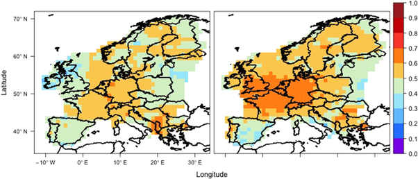
Figure 3. Spatial distribution of R2 in QR at the upper percentile 95th for MAM (left) and JJA (right).
Download figure:
Standard image High-resolution imageFigure 4 depicts the performance of the logistic models regression for the threshold 50 ppb. In general, models over south Europe perform better in spring than in summer, specifically in some regions such as Spain, North Italy, or South Balkan. However, the best performance is shown in central and northwest Europe, particularly in summer. Additional measurements of the goodness of the models have been analysed (supplementary material, section 3). The influence of LO3 is mainly noticed in south and northeast Europe (figure 5). However, there are some dominant meteorological drivers of ozone exceedances above 50 ppb: Tx, SR and RH. SR and RH are dominant in spring, while Tx becomes a significant driver of extreme ozone values in summer, especially in central, northwest Europe, and also in some specific southern locations. Both parameters show up as positive drivers of ozone extremes, though the influence of Tx is slightly higher in most of the grid-cells. These results show a seasonal and regional variation of drivers of extreme ozone conditions, which are mainly dominated by local meteorological parameters (i.e., RH, SR and Tx) in some specific regions (e.g., northwest and central Europe).
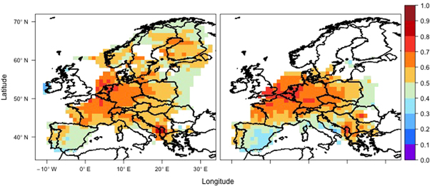
Figure 4. Spatial distribution of R2 in LR when analysing the limited value of 50 ppb, in MMA (left) and JJA (right).
Download figure:
Standard image High-resolution image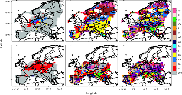
Figure 5. Spatial distribution of the most important driver (left), second most important (middle) and third most important (right) of ozone in LR for ozone exceedances (50 ppb) for both seasons: MAM (top) and JJA (bottom).
Download figure:
Standard image High-resolution image
4. Summary and conclusions
This study investigates the role of synoptic and local meteorological variability as a driver of surface concentrations of ozone, a toxic air pollutant. Additionally, by using a novel implementation of the JC97 classification, we are able to assess the effect of atmospheric circulation on a gridded ozone dataset. Three different regression models are employed to determine the drivers of maximum daily 8 h average ozone concentrations, as well as their extreme values as represented by their 95th percentiles, and exceedances of air quality guideline thresholds.
The drivers of surface ozone are identified during the model development using screening procedures that sequentially remove less significant drivers. The performance of the models is generally better in summer than spring. Geographically, the best performance is found in central and northwestern Europe (e.g., France, Belgium, Netherlands, Germany, Poland, Czech Republic, Austria or Switzerland). The inclusion of a one-day lag of ozone provides an additive value for predictions. Our results show that incorporating ozone persistence is particularly relevant in the southeast of Europe, especially in the Balkan Peninsula. However, we find that meteorological drivers account for most of the explained variance of ozone in most of the grid cells over central and northwest Europe.
One of the main drivers of ozone is the daily maximum temperature, which shows a positive relationship with ozone. We identify some specific areas where ozone is particularly sensitive to maximum temperature in summer (i.e. central and northwest Europe), which we suggest could be due to the effect of temperature on emissions of VOCs in this region which previous studies have been shown to be in a VOC-limited chemical regime. Maximum temperature becomes a key driver when ozone exceeds air quality target values (50 and 60 ppb). There is also considerable regional variation of the effect of maximum temperature: in southern and northern Europe, maximum temperature also appears as a driver but with a smaller effect. Relative humidity and solar radiation, negatively and positively related to ozone, respectively, appear as other relevant drivers, particularly in spring. Our results reveal some influence of the airflow indices on ozone in specific grid-cells, which suggests that the effect of wind speed and direction plays a role in influencing surface ozone concentration only in a small number of locations in Europe.
In conclusion, this statistical analysis provides insights into the strongest meteorological drivers of ozone, which play a significant role during the warmer months. Climate change is expected to influence regional weather conditions, such as warmer temperatures or stagnant conditions, and an increase in heatwaves (Russo et al 2015), which will likely adversely affect ozone levels and, consequently, air quality in Europe. With the regression models developed, we are able to identify regions, which may be particularly vulnerable to increased episodes of high ozone in the future, and where special attention should be paid to mitigation strategies. Our results imply that central Europe may be especially vulnerable to such increased episodes of high ozone in the future.
Acknowledgments
We thank Mark Lawrence and Peter J H Builtjes for valuable discussions during the manuscript preparation and are grateful for the constructive comments of two reviewers that helped to further improve the manuscript. J Sillmann is supported by the Research Council of Norway funded project CiXPAG (244551/E10).