

Abstract
The depletion of 14C due to the emission of radiocarbon-free fossil fuels (14C Suess effect) might lead to similar values in future and past radiocarbon signatures potentially introducing ambiguity in dating. I here test if a similar impact on the stable carbon isotope via the 13C Suess effect might help to distinguish between ancient and future carbon sources. To analyze a wide range of possibilities, I add to future emission scenarios carbon dioxide reduction (CDR) mechanisms, which partly enhance the depletion of atmospheric  already caused by the 14C Suess effect. The 13C Suess effect leads to unprecedented depletion in
  shifting the carbon cycle to a phase space in
  , in which the system has not been during the last 50 000 years and therefore the similarity in past and future
  (the ambiguity in 14C dating) induced by fossil fuels can in most cases be overcome by analyzing 13C. Only for slow changing reservoirs (e.g. deep Indo-Pacific Ocean) or when CDR scenarios are dominated by bioenergy with capture and storage the effect of anthropogenic activities on 13C does not unequivocally identify between past and future carbon cycle changes.
Export citation and abstract BibTeX RIS

Original content from this work may be used under the terms of the Creative Commons Attribution 3.0 licence. Any further distribution of this work must maintain attribution to the author(s) and the title of the work, journal citation and DOI.
1. Introduction
One of the side effects of anthropogenic CO2 emissions is the so-called (14C) Suess effect (Suess 1955), the depletion of the radiocarbon isotopic signature of atmospheric CO2 due to the injection of large amounts of 14C-free fossil fuels (Stuiver and Quay 1981). It has been shown with models (Caldeira et al 1998, Graven 2015) that by the end of the 21st century for most emission scenarios atmospheric  might be smaller than
  in surface and intermediate oceanic water masses. This would reverse the past and present day atmosphere-to-ocean gradient in
  and complicate conventional radiocarbon dating. For example, from the year 2050 onward fresh organic material might have the same 14C/12C ratio as samples from 1050 CE and earlier, making both past and future samples indistinguishable if analyzed by radiocarbon dating alone (Graven 2015).
Not yet mentioned in this previous analysis (Graven 2015) is the fact that 13C is also affected by anthropogenic CO2 emissions, since most of the released carbon has its origin in organic material, in which 13C is depleted with respect to 12C due to isotopic fractionation during photosynthesis (Lloyd and Farquhar 1994). Charles Keeling named this the 13C Suess effect (Keeling 1979), which has since then been widely observed in carbon reservoirs, e.g. in the atmosphere (Rubino et al 2013) and the surface ocean (Gruber et al 1999, Swart et al 2010, Schmittner et al 2013).
To project how emissions and therefore the Suess effects might develop in the future the international commitments to act against ongoing anthropogenic emissions need to be considered. Climate negotiations during the 21st Conference of Parties of United Nations Framework Convention on Climate Change in December 2015 in Paris have strengthened the political will to keep global warming caused by mankind under some agreed-upon thresholds (Iyer et al 2015), whose details are still a matter of debate (Knutti et al 2016). To meet such global warming thresholds, and to operate against a likely CO2 overshoot, not only a reduction in fossil fuel emissions (Rogelj et al 2013), but also some active CO2 removal from the atmosphere might be necessary (Smith et al 2016b) in order to achieve net zero emissions on the long-term (Rogelj et al 2015). Furthermore, once net zero emissions are achieved the rebound effect (Cao and Caldeira 2010), the outgassing of anthropogenic CO2 previously taken up by the ocean, might also urge mankind to implement negative CO2 emissions or carbon dioxide reduction (CDR) mechanisms in order to keep atmospheric CO2 at the desired concentration.
Model-based analysis of various CDR approaches are the subject of ongoing research. Within the most recent assessment of CDR (Smith et al 2016b) various different approaches have been compared with respect to their requirements in terms of energy, land, nutrient and water usages, their impacts on albedo and their costs. One of the CDR approaches analyzed in that study (bioenergy (BE) with carbon capture and storage (CCS), combined to BECCS) has already been implemented in some of the Representative Concentration Pathway (RCP) emission scenarios used for the most recent IPCC report (Meinshausen et al 2011, van Vuuren et al 2011). The magnitude of BECCS was up to 3.1, 1.2 and 0.2 PgC yr−1 in RCP2.6, RCP4.5 and RCP6.0, respectively, compensating for some of the fossil fuel emissions and leading in RCP2.6 to negative CO2 emissions at the end of this century (figure 1(A) inlet).

Figure 1. Future carbon cycle simulation results until year 2500 for all four emission scenarios (RCP2.6, RCP4.5, RCP6.0, RCP8.5) (Meinshausen et al 2011). (A) Total anthropogenic emissions rates E (sum of fossil fuel and land use change emissions). Net emissions (E–BECCS in PgC yr−1) for RCP2.6, RCP4.5, RCP6.0 are shown in the small inlet. (B) Contributions of land use change emissions to and prescribed CDR via BECCS already contained in the respective RCP scenarios. (C) Cumulative airborne fraction (AF):  with
with  change in atmospheric C content and
  the cumulative sum of emissions. (D) Simulated atmospheric CO2, black broken lines are the past reconstruction of CO2 (instrumental at Mauna Loa) (Keeling and Whorf 2005) and Law Dome ice core (Rubino et al 2013) or the mean of projected future concentrations of emission driven simulations within CMIP5 for the different RCP scenarios (Meinshausen et al 2011); (E) Simulated atmospheric
  and reconstructions (instrumental: Point Barrow, South Pole, Keeling et al 2001, ice cores: Law Dome and WAIS Divide, Rubino et al 2013, Bauska et al 2015); (F) Simulated atmospheric
  including in black the reconstructed radiocarbon bomb peak (Hua et al 2013); (G) Simulated mean pH of the surface ocean.
Download figure:
Standard image High-resolution imageI will here have a look at potential changes in the carbon isotopes in the future and analyze how the 13C Suess effect might help to solve the proposed future radiocarbon dating conundrum caused by the 14C Suess effect. For this aim I will extend the analysis of the emission scenarios to the year 2500 using the well tested carbon cycle box model BICYCLE (Köhler et al 2005), which is described in detail in the supplementary material. The extensions of the RCP emissions scenarios beyond the year 2100 were labeled the Extended Concentration Pathways (ECPs) (Meinshausen et al 2011). However, for reasons of simplicity I here address the emission scenarios as 'RCP', no matter if it concerns changes until or after the year 2100. I will also incorporate how the carbon cycle might be further affected by some CDR methods discussed nowadays to cover an as wide as possible range of potential changes in 13C and 14C. Finally, I set the simulated future dynamics in the carbon isotopes into perspective of what is known from paleo data (and modeling) covering the last 50 000 years.
2. Simulation scenarios
I use the historical anthropogenic carbon release (1765–2005) from both fossil fuel emissions (including cement production) and land use changes (figure S1A) as contained in the extended version of the RCP emission scenarios (Moss et al 2010, Meinshausen et al 2011), which proposed carbon emissions from 2006 onward until the year 2500 (figure 1(A)). The historical emission fluxes contained in the RCP scenarios (Meinshausen et al 2011) are slightly smaller in the 2nd half of the 20th century than in those previously published (Houghton 2003) due to some downward correction of the land use emission fluxes. Assumptions then have to be made on the isotopic signature of the emissions (figure S1B): the  signature of fossil emissions is taken from reconstructions between 1765 and 2011 and kept constant at its 2011 value thereafter (Andres et al 2000, 2015), while that from land use change is internally calculated from the atmospheric
  value using the isotopic fractionation during C3 photosynthesis by −19‰. Similarly, the 14C signature from land use emissions is derived using twice the named isotopic fractionation for
  , while fossil fuels are assumed to contain no 14C. I only consider CO2 emissions, all other anthropogenic emissions contained in the RCP scenarios are neglected.
The 14C production rate is prescribed before 1950 CE (Roth and Joos 2013) varying around a mean production rate of 440 mol per year, kept constant thereafter with individual years in the 1950ies to 1970ies with high peaks in 14C production caused by nuclear bomb testing (Naegler and Levin 2006) (figure S1C). Potential impacts of 14C production from the nuclear industry (Graven and Gruber 2011, Graven 2015) are tested with sensitivity runs (see supplementary material for details on 14C production rate). All simulations are started in year 10 000 BP to allow the 14C cycle to adjust to variable production rates.
For model evaluation (supplementary material) the simulated time series of atmospheric CO2,  and
and  are then compared with historical data from both ice cores and instrumental records (figure S2), but also with the proposed atmospheric CO2 concentrations of the RCP emission scenarios (Moss et al 2010, Meinshausen et al 2011) that should be taken as radiative forcing time series in the CMIP5 model intercomparison project.
Additionally I investigate three different methods of CDR, (a) bioenergy with capture and storage (BECCS), (b) direct air capture (DAC), and (c) ocean alkalinization or enhanced weathering (EW), which all interact with the carbon cycle in completely different ways. I prescribe the strength of these three methods in order to linearly reduce net carbon emissions from 2021 onward until an annual net removal of 5 Pg C yr−1 is achieved in the year 2050, and maintained thereafter. Alternatively, after year 2070 the 5 Pg C yr−1 net CO2 removal would cease (scenarios BECCSs, DACs and EWs), and the simulations would continue. In DAC carbon is extracted from the atmospheric pool and assumed to be permanently stored in some geological reservoir without any further exchange with the atmosphere-ocean-terrestrial biosphere subsystem of the carbon cycle. The storage is similar in BECCS, but the extraction of carbon is based in biologically produced organic carbon, implying that isotopic fractionation during photosynthesis took place first, having a net effect on the carbon isotopes, and making BECCS similar to a land use change scenario with negative emissions. In EW an enhanced weathering or ocean alkalinization flux is calculated that approximates the desired CO2 removal: 1 mol of desired CO2 removal triggers the input of 1 mol of bicarbonate ion ( ) into the surface ocean, which would be the product of any man-made EW by enhanced silicate weathering that changes both the carbon content and the alkalinity in the ocean and ultimately the CO2 uptake capacity of the world oceans. In practical terms the molar input of
  can be related to the necessary amount of silicate rocks that needs to be dissolved by the relevant net chemical dissolution equations, e.g. 1 g of olivine (Mg2SiO4 with about 140 g mol–1) would lead to a theoretical input of
  of
of  (for details see Köhler et al 2010, Griffioen 2016). Any second order effects of enhanced silicate rock weathering that might occur due to changes in the biological pump (Köhler et al 2013, Hauck et al 2016) are ignored here.
The isotopic signature of fluxes related to BECCS, DAC and EW are consistently calculated within the model: both the CO2 extracted within BECCS and DAC and the influx of  into the surface ocean during EW contain the
  and
and  signatures of the atmospheric reservoir during the relevant time step (additionally within BECCS isotopic fractionation by −19‰ due to photosynthesis is considered). The differences in the isotopic signatures of the RCP and CDR fluxes are the reason why both the emission and the CO2 removal fluxes need to be prescribed individually, and not only as one net flux. The size of BECCS as assumed in RCP2.6, RCP4.5, and RCP6.0 in the 21st century is assumed to stay constant on its 2100 level thereafter (figure 1(B)).
3. Results and discussions
My discussion of carbon cycle results is focused on the RCP8.5 emission scenario and subsequent CDR approaches diverging from it. However, the results for the other scenarios (RCP2.6, RCP4.5, RCP6.0) are included in the figures and the effects on the carbon isotopes in them is contained in my analysis of the combined Suess effects.
3.1. Carbon cycle dynamics
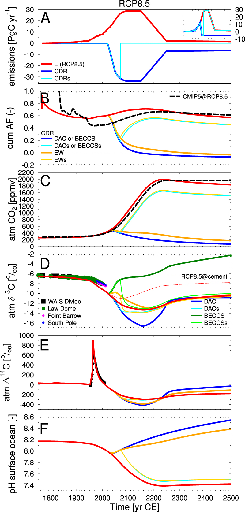
In the RCP8.5 emission scenario mitigation efforts start late leading to anthropogenic emission rates of up to nearly 30 Pg C yr−1 around year 2100 with an assumed linear reduction between 2150 and 2200 to a constant emission rate of 1.5 Pg C yr−1 until year 2500. (figure 2(A)). These emissions would result in a rise in atmospheric CO2 concentration from present day 400 ppmv to ∼2000 ppmv after year 2200 in both the CMIP5 scenarios (Meinshausen et al 2011) and my carbon cycle simulations (figure 2(C)). The global warming and ocean acidification connected with such a rise in the most important anthropogenic greenhouse gas would be severe leading in my simulations to a temperature rise of 5–6 K (figure S3) and a drop in mean surface ocean pH by 0.8 units (from 8.2 to 7.4) (figure 2(F) inlet).

Figure 2. Carbon cycle simulation results from pre-industrial times until year 2500. Results are based on RCP8.5 emission scenario (Meinshausen et al 2011) including carbon dioxide reduction (CDR) via bioenergy and carbon capture and storage (BECCS), direct direct air capture (DAC) and enhanced weathering (EW). BECCS and DAC differ only in  , changes in
  are on the order of a few permil only and negligible. (A) Emission rate E of RCP8.5 in the extended scenario until 2500 and the negative emissions of CDR approaches. Small inlet sketches the net emissions (E–CDR in PgC yr−1). (B) Cumulative airborne fraction (AF):
  with
with  change in atmospheric C content and
  the cumulative sum of emissions. (C) Simulated atmospheric CO2, black broken line is the past reconstruction of CO2 (instrumental at Mauna Loa) (Keeling and Whorf 2005) and Law Dome ice core (Rubino et al 2013) or the mean of projected future concentrations within CMIP5 for RCP8.5 (Meinshausen et al 2011); (D) Simulated atmospheric
  and reconstructions (instrumental: Point Barrow, South Pole, Keeling et al 2001, ice cores: Law Dome and WAIS Divide, Rubino et al 2013, Bauska et al 2015). RCP8.5@cement is a sensitivity study in which the source of the fossil fuel emission is slowly shifting from today 6% to 100% cement in year 2250. Cement has a
  signature of 0‰. (E) Simulated atmospheric
  including in black the reconstructed radiocarbon bomb peak (Hua et al 2013). (F) Simulated mean pH of the surface ocean.
Download figure:
Standard image High-resolution imageWithin the hypothetical CDR scenarios investigated here, net emissions are reduced even faster than in the other RCP emission scenarios assuming negative net emissions from year 2040 onward (figure 2(A)) and therefore broaden the range of possible future scenarios. The carbon extraction achieved in these CDR simulations might be unrealistically high, however, my interest here lies in showing potential maximum impacts on the carbon isotopes and not to investigate the most plausible scenario.
The cumulative airborne fraction (AF) of the anthropogenic emissions E (Pg C yr−1), here defined as the ratio in the difference in atmospheric carbon pool (with respect to the pre-industrial values in year 1765) over the cumulative sum of E, stays in my simulations around 0.6 (figure 2(B)). Cumulative AF calculated from emission driven CMIP5 data are before year 1830 larger than 1, probably due to carbon cycle internal variability not driven by the yet small anthropogenic emissions. In the 21st and 22nd centuries they are slightly smaller than in my simulations. This difference is explained with the passive (=constant) terrestrial carbon pools in my simulations which neglects the terrestrial carbon sink found in the historical data (Le Quéré et al 2015). I refrain from showing results with active (=variable) terrestrial carbon cycle, since for atmospheric CO2 concentrations well above 500 ppmv, the CO2 fertilization implemented in my simple model is much too large, when compared with CMIP5 models, leading, due to the massive buildup of terrestrial carbon, to unrealistically low atmospheric CO2 concentration (Köhler et al 2015). I here restrict simulation results to those obtained with an atmosphere-ocean only setup of the the carbon cycle, which on the long run agree in the atmospheric carbon pools with those of the CMIP5 results, although the still existing uncertainty in the land carbon cycle, partly due to an overestimation of the CO2 fertilization (Smith et al 2016a), or due to uncertainties in the nitrogen cycle (Meyerholt et al 2016) might indicate that CMIP5 results are also not perfect. On the long run the cumulative AF and atmospheric CO2 of my simulations converge with those based on CMIP5, indicating a small long-term influence of the terrestrial carbon sink in models contributing to CMIP5 (figures 1(C) and 2(B)). Simulations including terrestrial carbon storage changes would result in smaller simulated atmospheric CO2, smaller AFs, and less depleted atmospheric  . Therefore, the historical 13C Suess effect is better matched by using an active terrestrial carbon cycle (figure S2B), while the effect on the historical 14C Suess effect reduces the offset between model and data, but has negligible impact on the 14C dynamic (figure S2C).
All CDR methods have a permanent impact on atmospheric CO2 concentrations and on surface ocean pH (figures 2(C), (F)). Even in the scenarios BECCSs, DACs and EWs, in which CDR is stopped after some decades (here in year 2070) the simulated CO2 concentrations (and surface ocean pH) do not reach the values obtained without CDR. The assumed CDR scenarios would eventually lead to a cumulative AF of zero, implying that an amount of CO2 identical to the sum of all anthropogenic CO2 emissions has been extracted from the carbon cycle again and atmospheric CO2 concentration starts to fall below pre-industrial values.
3.2. Carbon isotopes: the 14C and 13C Suess effects
The carbon isotopes of atmospheric CO2 are both depleted by the massive injection of anthropogenic emissions, since fossil fuels are 14C-free and contain with about −24 to −29‰ a  signature (Andres et al 2000, 2015) that is 19‰ lighter than the
  signature of the atmospheric CO2 itself (figure S1B). Additionally, the radiocarbon cycle is penetrated by the bomb-14C emissions in the second half of the last century (Naegler and Levin 2006) leading around 1965 to atmospheric
  values of up to +700 ± 200‰ in the data (Hua et al 2013) and of +900‰ in my simulations (figure 2(E)) (see supplementary material for further details).
Atmospheric  then drops around 2150 to −300‰ in RCP8.5 and to −415‰ in all CDR approaches. This most depleted
  signature of −415‰ is identical to that of a 4300 year old carbon sample (figure 3(A)). Depending on the assumed CDR method
  of atmospheric CO2 drops at the same time to values of (RCP8.5) −13.3‰, (EW) −12.6‰, or (DAC) −16.6‰ (figure 2(D)). For BECCS
  of atmospheric CO2 returns to its pre-industrial value of −6.5‰ in year 2150 and rises thereafter to values up to −2‰. Here, the difference of how the CDR methods modify the carbon cycle has a significant impact on the resulting atmospheric
  signature: BECCS operates as negative land use change, therefore reversing the 13C Suess effect. In scenario EW alkalinity is added to the ocean. The isotopic fractionation within the dissolved inorganic carbon (DIC) in the ocean and therefore of the ocean-atmosphere gas exchange depends directly on the concentration of
  and
and  , two of the chemical species of DIC. However, the concentrations of these species change with a rise in alkalinity to allow a larger oceanic CO2 storage. Therefore, the isotopic fractionation during gas exchange indirectly depends on the surface ocean alkalinity (Zeebe and Wolf-Gladrow 2001) and is in detail implemented in BICYCLE similarly as in other models (Ridgwell 2001).

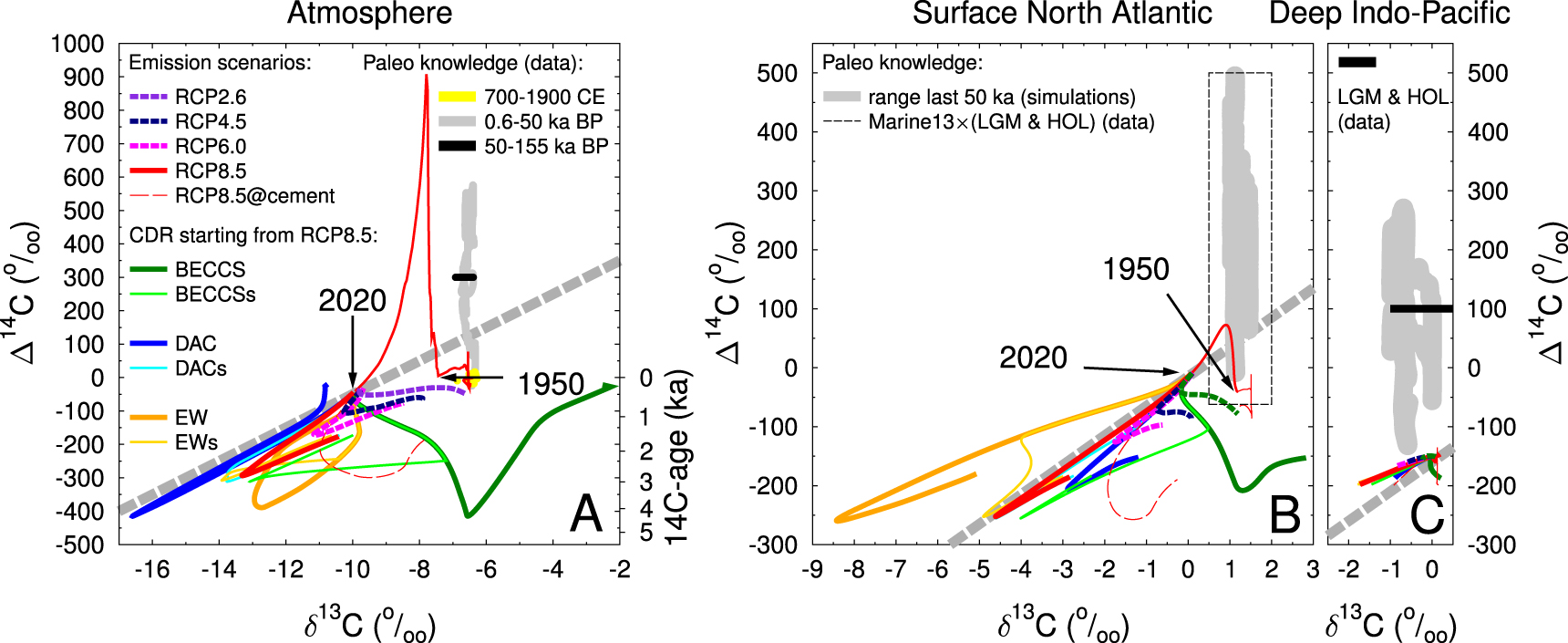
Figure 3. Analysis of the combined Suess effects on both 14C and 13C. Scatter plot of simulated  versus
  (A) atmosphere, (B), (C): end-members within the ocean (surface North Atlantic, deep Indo-Pacific) showing the historical and future Suess effects and the influence of bomb-14C, future CO2 emissions and carbon dioxide reduction (CDR) approaches (BECCS, DAC, EW) on both variables. Also included in dotted lines are results for RCP2.6, RCP4.5 and RCP6.0, which all contain a prescribed contribution of BECCS (see figure 1 for details). The right y-axis in panel (A) also provides, similarly as before in Graven 2015, a conventional calculated 14C-age =
  for all
  values below zero (1 ka = 1000 years). For comparison, also the available paleo knowledge is added: (A) Atmospheric
  from ice cores (700–1900 CE: WAIS Divide ice core, Bauska et al 2015; further back in time: spline through ice core compilation, Eggleston et al 2016) and
  from IntCal13 (Reimer et al 2013), for 50–155 ka BP plotted with fixed
  ‰; In the ocean I show the data range obtained from sediment cores in
  (Peterson et al 2014) obtained for the Last Glacial Maximum (LGM) and the late Holocene (HOL) for (B) the range of surface ocean
  contained in Marine13 (Reimer et al 2013) or (C) for a fixed value of
  ‰. Additionally, the range in both isotopes in previously published (imperfect) simulations using the BICYCLE model covering the last 50 000 year (50 ka) is shown (upper limit of scenario S3x (14C production rate based on 10Be) and lower limit of scenario S4x (14C production rate based on reconstructions of the geomagnetic field strength GLOPIS-75) as used before in Köhler et al 2006). The gray broken line in all subplots crosses values for year 2020 with a slope m = 50 (see text for further explanation).
Download figure:
Standard image High-resolution imageWhen  and
and  are plotted against each other it clearly becomes evident that the Suess effects on both isotopes will in the future bring the isotopic carbon cycle into a regime in which it has not been during at least the last 50 000 years. The historical Suess effect before 1950 (−0.7‰ in
  and −20‰ in
  ) already shifted the atmospheric variables away from its natural state (figure 3(A)). The atmospheric
  simulated in response to the bomb-14C injection led to 0 to +900‰, slightly larger than the range of −25-to- +575‰ that has been reconstructed for the pre-industrial 50 000 years from various archives (Köhler et al 2006, Reimer et al 2013). Already the historical emissions from 1950 onward including the foreseeable emissions until 2020 shift the atmospheric
  by another −2‰. In most scenarios a further depletion in both carbon isotopes takes place in the near future. At the extreme, values of
  and
and  are reached in the atmospheric carbon reservoir. The exceptions to this rule are scenarios in which BECCS plays a dominant role, also implying that RCP2.6 has a different dynamic in the carbon isotopes than the other RCP scenarios. EW would first lead to a small rise in
  but on the long run also to a depletion. In BECCS the simulated
  on the long run is higher than what is known from the paleo record. Most scenarios might, after having a maximum depletion in the isotopic phase space, return to less extreme anomalies in both isotopes, only RCP2.6 returns in the
  -scatter plot back to conditions seen in pre-industrial times or found in the paleo simulations or reconstructions.
To analyze how the carbon isotopes in the ocean might change due to the Suess effects I focus on the two end-member in the oceanic carbon cycle: (a) North Atlantic surface waters, where North Atlantic Deep Water formation occurs and a dominant part of deep ocean water masses have last contact with the atmosphere and (b) the deep Indo-Pacific, in which the oldest, most  -depleted water masses are found. A similar pattern as found in the atmosphere emerges in the North Atlantic surface waters, although with smaller amplitude (figure 3(B)): the bomb-14C spike is found with slightly more than +100‰, the 13C Suess effect leads until 2020 to a reduction in
  by nearly −1.5‰, and all scenarios but RCP2.6 enter uncharted waters in the
  phase space. Clearly seen is also that the rising ocean alkalinity in the EW CDR method leads to a more depleted surface ocean
  , explaining the lower isotopic fractionation (less depletion) in the atmospheric
  record and the special dynamics for BECCS leading to
  of nearly +3‰. An overlap of the historical and future simulations with the data range spanned by paleo data (Reimer et al 2013, Peterson et al 2014) and paleo simulations (Köhler et al 2006) covering the last 50 000 years is only obtained for the bomb-14C spike. Also note, that these paleo simulations, performed with a previous version of the same model, were imperfect, since they were not able to explain the full decline in atmospheric
  found in the paleo reconstructions (Reimer et al 2013).
The simulated changes in the deep Indo-Pacific during the next five centuries are much smaller than for the surface ocean (figure 3(C)). Until 2020 the Suess effects or even the 14C-bomb spike are not detectable in this reservoir, however the effect of further anthropogenic emissions will over the course of the simulations found its way to this most remote ocean reservoir and both Suess effects will then be visible there. The simulated future trends in the deep Indo-Pacific  have some overlap with the range of reconstructed
  , however, the knowledge on deep ocean
  is still limited. While my previous (imperfect) simulations suggest that deep Indo-Pacific
  was always higher than −150‰ throughout the last 50,000 years, the limited available deep ocean
  reconstructions show a different picture (Ronge et al 2016):
  -values as low as −200‰ are found in waters above 2000 m and below 4300 m water depth in the South Pacific with some water masses in between (and in intermediate depths of ∼600 m around the Galapagos Islands (Stott et al 2009) having during the last 25 000 years a
  signature as low as −600‰. This would imply that for most of the RCP emission scenarios the deep Pacific data in the
  phase space might already have been obtained in some form during glacial conditions in the past. These most recent deep Pacific data with low
  signature (Ronge et al 2016) are not yet completely understood. It is not yet clear how wide-spread this water mass is and the explaining hypothesis put forward so far suggests the release of 14C-free CO2 from hydrothermal activities along mid-ocean ridges during sea-level low stand in glacial times. This would imply that the deep glacial ocean would contain, in addition to the fossil fuel emissions into the atmosphere, another source of 14C-free carbon. The interpretation of deep ocean carbon isotopic signatures might therefore be not yet straight-forward.
Simulation results for other surface ocean reservoirs are qualitatively similar to the North Atlantic surface end member discussed in detail above (figure S4), allowing in surface reservoirs to use the 13C Suess effect to distinguish past from future carbon fluxes. Interestingly, the largest oceanic anomalies in  are obtained in the surface equatorial Atlantic Ocean (figure S4B) with
  falling down to −13‰ for EW scenarios, probably caused by the way the EW fluxes are prescribed. These fluxes enter the surface ocean only in the equatorial regions, with 50% each routed in the Atlantic and Indo-Pacific. Combined with the smaller size of the Atlantic basin, the effect of EW on the local carbon cycle is more pronounced in the Atlantic than in the Indo-Pacific. Since the prescribed water mass fluxes to the surface North Pacific area are all sourced in deep ocean regions,
  in this area follows in the EW scenarios the dynamics seen in the atmosphere (less depleted than in RCP8.5, figure S4F). Carbon isotopic dynamics in the deep ocean of the Atlantic (figure S4C) and to some extend in the Southern Ocean (figure S4E) depart from known data ranges in the past. My approach to disentangle past from future carbon cycle changes therefore seemed also to be applicable to data from these deep ocean reservoirs. Further regional details are better obtained with spatially higher resolved models.
Fossil fuel fluxes contain also emissions from industrial processes, namely cement production. The  signature of fossil fuels therefore depends on the source mix and ranges from 0‰ (cement production) to −44‰ (natural gas) (Andres et al 2000). About 6% of the CO2 emissions summarized as fossil fuels in year 2014 have been from cement production (Le Quéré et al 2015). In my standard scenarios I assume that the source mix (and therefore the
  signature of fossil fuels) remains the same from year 2011 onward. In one scenario (RCP8.5@cement) I test the effect when cement production would slowly become the one and only source of the fossil fuel emissions in year 2250 (evolution of
  of fossil fuels shown in figure S1B). Simulated
  values would then be less depleted than in our standard simulations (figure 2(D)), but isotopic values would still be outside of their ranges known from the past (figure 3), and the overall conclusion would therefore not be affected by such a rise in the relative importance of cement in the source mix of future fossil fuel emissions.
4. Conclusions
When considering not only the 14C Suess effect but also the 13C Suess effect the future changes in the carbon isotopes in the atmosphere and the neighboring reservoirs (surface ocean, to some extend relatively fast ventilated water masses of the deep ocean, but also terrestrial biosphere) follow a distinct pattern that makes them distinguishable from variability in the past. This study is after the initial modeling study (Keeling 1979) one of a few approaches (e.g. Jahn et al 2015) in which both Suess effects are considered together. Simulation studies typically focus on either the 14C Suess effect (Caldeira et al 1998, Graven 2015) or 13C Suess effect (Gruber et al 1999, Tagliabue and Bopp 2008, Schmittner et al 2013). Changes in the carbon isotopic signature can be approximated from theory by considering that the injection of 14C-free fossil fuels with a  signature of −28‰ leads to a carbon influx that differs from the present day atmosphere by
  ‰ and
‰ and  ‰. These differences are equivalent to a linear change with a slope
  in the
  phase space as indicated by the broken lines in figures 3 and S4. The realized simulations that do not contain CDR due to BECCS or EW, nearly meet this theoretical expectation.
I therefore propose that measuring 13C in parallel to 14C measurements will enable researchers to distinguish the future from the past in radiocarbon. This approach should be applicable for carbon reservoirs that are in reasonable fast exchange with the atmosphere to allow any Suess effect to be visible in the data sets. For data from deep ocean sites, especially from the Indo-Pacific, the observed future variability in the carbon isotopes might be too small to identify a clear excursion from past data ranges. If a 14C-age falls within the range of 0 to 5000 years (corresponding to  in the atmosphere of approximately 0 to −450‰) a crosscheck on the 13C Suess effect is necessary (figure 4). Here, isotopic fractionation during photosynthesis needs to be taken into account, if the relevant probe was derived for organic carbon. If the carbon cycle has been heavily perturbed by both Suess effects, the probe has its origin (age) within this or future centuries. If no 13C Suess effect can be detected then the relevant carbon is of ancient origin, e.g. it had its last contact with the atmosphere in the past before fossil fuels perturbed the carbon cycle. For the exception that a large contribution of CDR is obtained via BECCS further evidences might be necessary since the carbon cycle might then not leave the
  –δ13C-space known from historical and paleo reconstructions. I am aware that this isotopic fractionation during photosynthesis depends on various factors and might itself lead to a wide range of
  within any organic material (Lloyd and Farquhar 1994), even without any perturbations of the 13C Suess effect. Therefore, expert knowledge on the expected natural range of
  within the any organic material is certainly necessary to make this final conclusion.

Figure 4. Decision tree how to distinguish ancient carbon from carbon which requires an age marker from future times. The combination of radiocarbon dating and how  needs to leave its natural range due to the combined 14C and 13C Suess effects with examples for the atmospheric reservoir are given. For cases in which CDR by a large contribution of BECCS is realized (e.g. as in RCP2.6) the carbon isotopic signatures might return back to pre-industrial values. For these cases further not yet identified evidence is necessary to distinguish ancient from future carbon. For slow changing reservoirs, e.g. the deep Pacific, changes for the future overlap with past data ranges, so a clear identification of ancient versus future carbon is not possible.
Download figure:
Standard image High-resolution image
Earth system models contributing to CMIP5 including an active terrestrial biosphere might reduce uncertainties in the simulated future carbon cycle dynamics. The general pattern found here with a simplified carbon cycle model that the 13C Suess effect might be used to distinguish between past and future carbon sources, however, is robust and should not change if investigated with more complex models.
Acknowledgments
The design of the CDR scenarios was motivated by initially proposed scenarios within the CDR-MIP project. Thanks to the RCP core group and Heather Graven for providing data on the amplitude of BECCS within the RCP scenarios. I thank Dieter Wolf-Gladrow and Gregor Knorr for helpful comments. Simulation results are available from the data base PANGAEA (doi: 10.1594/PANGAEA.868739).