

Abstract
Land surface models (LSMs) must accurately simulate observed energy and water fluxes during droughts in order to provide reliable estimates of future water resources. We evaluated 8 different LSMs (14 model versions) for simulating evapotranspiration (ET) during periods of evaporative drought (Edrought) across six flux tower sites. Using an empirically defined Edrought threshold (a decline in ET below the observed 15th percentile), we show that LSMs simulated 58 Edrought days per year, on average, across the six sites, ∼3 times as many as the observed 20 d. The simulated Edrought magnitude was ∼8 times greater than observed and twice as intense. Our findings point to systematic biases across LSMs when simulating water and energy fluxes under water-stressed conditions. The overestimation of key Edrought characteristics undermines our confidence in the models' capability in simulating realistic drought responses to climate change and has wider implications for phenomena sensitive to soil moisture, including heat waves.
Export citation and abstract BibTeX RIS

Original content from this work may be used under the terms of the Creative Commons Attribution 3.0 licence. Any further distribution of this work must maintain attribution to the author(s) and the title of the work, journal citation and DOI.
1. Introduction
Droughts are major natural hazards with widespread impacts on humans and ecosystems. Severe drought events have been experienced in the last decade across different regions of the world, including Australia (van Dijk et al 2013), the Amazon (Marengo et al 2008, Lewis et al 2011) and North America (Seneviratne 2012, Griffin and Anchukaitis 2014), with consequences for water resources management and ecosystem productivity (Dai 2011). The frequency and magnitude of droughts are expected to increase regionally in the coming decades due to climate-change driven changes in precipitation and evapotranspiration patterns (Dai 2011, 2013, Sheffield et al 2012, IPCC 2013, Orlowsky and Seneviratne 2013, Prudhomme et al 2014). Due to the vulnerability of many regions to drought, it is crucial that land surface models (LSMs) correctly characterise these phenomena as a first step to the provision of reliable projections of future water availability across the land surface.
LSMs have wide-ranging applications, varying from providing the lower boundary for climate and weather prediction models (Pitman 2003) to operational water resource monitoring (e.g. Crow et al 2012). LSMs also underpin studies investigating historical (Sheffield and Wood 2008, Wang et al 2009, Dai 2011) and future (Burke and Brown 2008, Dai 2013, Prudhomme et al 2014) changes in drought and as such, are a key tool for understanding and quantifying these extreme events. The capability of LSMs to capture droughts has not been widely evaluated, with many model inter-comparison studies instead focusing on seasonal to annual scale averages (Henderson-Sellers et al 1995, Best et al 2015). Some recent studies have identified deficiencies in individual LSMs in simulating carbon and water fluxes during seasonal-scale droughts in a range of climates and ecosystems (Prudhomme et al 2011, Li et al 2012, Powell et al 2013, Tallaksen and Stahl 2014, De Kauwe et al 2015, Ukkola et al 2016, Whitley et al 2016). For example, the Community Atmosphere Biosphere Land Exchange (CABLE; Wang et al 2011) LSM has been shown to systematically underestimate site-scale evapotranspiration (ET) during anomalous dry conditions such as the 2003 European drought (De Kauwe et al 2015) and regular dry seasons, such as those observed in savannas (Whitley et al 2016). The Joint UK Land Environment Simulator (JULES; Best et al 2011) LSM has been shown to enter hydrological (streamflow) droughts too slowly, whilst overestimating ensuing drought duration and severity. JULES and several other LSMs, including ORCHIDEE (Organising Carbon and Hydrology in Dynamic EcosystEms; Krinner et al 2005), have also been found to overestimate the frequency of hydrological droughts due to the over-sensitivity of models to short-term precipitation variability (Prudhomme et al 2011, Tallaksen and Stahl 2014).
These findings have pointed to limitations in specific LSMs used for characterising the magnitude, duration and frequency of droughts. However, previous studies have commonly relied on a single LSM and as such, it is unclear if the biases identified in previous studies are systematic amongst LSMs, or rather due to how individual models represent and parameterise key processes. We therefore evaluate eight unique LSMs (and 14 model versions in total) in simulating ET during water-stressed conditions across six flux tower sites with pronounced seasonal-scale dry periods. In contrast to large-scale applications of LSMs, flux tower measurements offer direct observations of energy and water fluxes at time scales ranging from minutes to multiple years. As such, they offer excellent opportunities for improving process-level understanding of LSMs, whilst minimising uncertainties in forcing and evaluation data that would otherwise undermine our ability to reliably evaluate model performance.
2. Methods
Many definitions of drought exist, including meteorological (precipitation (P)), hydrological (streamflow) and ecological (soil moisture) drought (Sheffield and Wood 2011, Van Loon et al 2016). Here, we use ET to evaluate what we term 'evaporative drought' in LSMs since (a) this is the water availability variable directly measured by flux towers and, (b) it provides access to simulations at a range of sites by many LSMs that took part in the Protocol for the Analysis of Land Surface Models (PALS) Land Surface Model Benchmarking Evaluation Project (PLUMBER; Best et al 2015). The use of ET also allows for the evaluation of the contribution that LSMs can make to enhancing or dampening drought characteristics that are imposed by prevailing meteorological conditions. This 'evaporative drought' (Edrought hereafter) is not provided as another formal definition of drought. Rather, we use the term to encompass regularly occurring dry seasons as well as anomalous dry periods as these both serve as useful references for model performance during water-stressed periods. As such, we do not rely on existing evaporative drought indices (e.g. Narasimhan and Srinivasan 2005, Anderson et al 2011, Hobbins et al 2016) but formulate an alternative index based on similar principles.
We employ three metrics to quantify the duration, magnitude and intensity of Edroughts. We define the Edrought threshold (q15) empirically as the annual 15th percentile value of observed daily ET. Unlike other hydrological variables commonly used to characterise droughts, low ET does not necessarily result from low water availability but can also follow from low incident energy supply to vaporise water. To avoid falsely characterising days with low radiation supply as periods of drought, we use the ratio of actual to potential ET (PET) as an additional constraint. Low actual ET (AET) compared to PET indicates water-limited conditions whereby evaporative demand cannot be met by available water supply. We standardise the evaporative ratio (ER) by annual mean daily PET ( mm d−1) to avoid characterising days with low PET (e.g. during high latitude winter) as drought:

where Ea and Ep are the daily actual and PET (mm d−1), respectively. We calculated daily PET using the Priestley–Taylor equation (Priestley and Taylor 1972) based on observed shortwave radiation and air temperature following Gallego-Sala et al (2010). We also repeated the analysis using the Penman PET equation (Penman 1948), which also includes the effects of wind and humidity, but our findings were robust to the choice of PET method.
Edrought duration (D) was determined separately for each model as the number of days with daily ET below the q15 value and the ER below its observed annual 15th percentile value at each site. Each Edrought event was defined as a period of 14 or more consecutive Edrought days. We examined the impact of different thresholds for q15 and ER; these did not qualitatively impact our conclusions. Subsequently, Edrought magnitude (M) was calculated separately for each event as the cumulative sum of the difference between q15 and daily ET (E) during the Edrought days (d):

where i is the Edrought start date and j the end date. We term this as the 'cumulative deficit' following Sheffield and Wood (2011). Finally, Edrought intensity (I) was determined as the difference between q15 and the minimum daily ET during each Edrought event:

All metrics were determined separately for each model and each site. 14 day running mean ET was used for all analyses.
Model simulations for the 13 LSM versions were acquired from PLUMBER (Best et al 2015) and we added a version of the CABLE LSM (Decker 2015) for this study. The models were forced with observed half-hourly meteorology at each site, using an identical spin-up protocol. The models were not calibrated locally at the sites. Whilst calibration would likely improve model performance, it may not necessarily reflect the skill of LSMs when run at the larger scales they are typically developed for. Instead, site calibration may mask significant deficiencies in LSMs and lead to parameter values that perform well at the calibration site, but are likely to be over-fitted for the intended broad scale application. A full description of the LSMs and modelling protocols is available in Best et al (2015) but a summary of the participating LSMs is provided in table S1. The PLUMBER archive has simulations for 20 flux tower sites; we focus our analysis on six of these sites with pronounced seasonal drought periods during periods of high potential evaporation. For completeness, we provide results for the remaining sites in figure S1. Note we exclude Sylvania because precipitation forcing was erroneous and El Saler 2 which is an irrigated site (Haughton et al 2016). The drought metrics were calculated using all available years, ranging from two to seven years for the selected sites. The six sites discussed in detail provide a reasonably distributed global sample and cover a range of vegetation and climate types (figure S2; table S2). They also exhibit the key process-level strengths and weaknesses that can be identified in the overall PLUMBER archive and therefore provide a good guide to model performance across the whole 20 sites used in Best et al (2015).
3. Results
Figure 1 shows LSM simulations for individual years across the six sites and the associated observations for ET and precipitation to illustrate typical LSM behaviour at these sites. There are clear deficiencies in simulations of ET at most sites. At Amplero, most models agree with observations in the early part of the year but as rainfall declines, the LSMs diverge from each other considerably. One model reduces ET dramatically in June (ISBA-3L), others decline strongly in July (e.g. Noah 2.7, ISBA-dif and CABLE-2.0) while several models continue to closely match the observations to the end of the year (CABLE-SLI, CABLE-GW and Mosaic). In September, modelled ET ranges from near zero to ∼3 mm d−1. At Espirra and Blodgett, a similar result is obtained, with a divergence in the LSMs with ET again ranging from near zero to ∼3 mm d−1 and ∼4 mm d−1 in July, respectively. Almost all LSMs underpredict ET compared to observations in July at Howard Springs and Mopane. At Palang some LSMs capture observed ET well, while others show similar behaviour to Amplero.
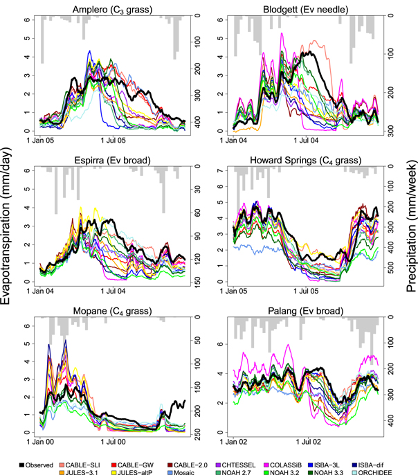
Figure 1. Simulated and observed evapotranspiration during an example one-year period. The ET time series show the 14 d running mean from January to December. The grey bars show 7 d precipitation totals.
Download figure:
Standard image High-resolution imageWe next quantify these qualitative descriptions of LSM biases using all available years. Figure 2(a) shows the Edrought duration simulated by each LSM. On average, the LSMs simulated 58 Edrought days per year across the six sites, compared to 20 d in the observed ET flux data. Model estimates ranged from 22 (ORCHIDEE) to 103 (Noah 3.2) Edrought days per year and, as such, all the participating LSMs overestimated Edrought duration when averaged across the six sites. The largest error in Edrought duration was simulated for the Palang site (on average 74 d more than observed). The smallest error was simulated in Mopane (15 d more than observed).
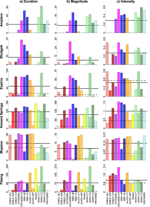
Figure 2. Simulated and observed (a) Edrought duration (number of Edrought days per year), (b) Edrought magnitude (cumulative deficit; mm yr−1) and (c) Edrought intensity (mm) at the six flux tower sites. Individual model estimates are shown as coloured bars, observations as the dotted line and the mean of all models as the solid line.
Download figure:
Standard image High-resolution imageWe then evaluated the LSMs for simulating Edrought magnitude using the cumulative deficit metric (figure 2(b)). The average simulated annual total cumulative deficit was 37 mm compared to 4 mm observed, an overestimation of around 700%. This is partly due to the LSMs overestimating Edrought duration. When averaged to daily Edrought magnitude, the simulated mean magnitude was 0.39 mm d−1 compared to the observed 0.20 mm d−1. As such, the LSMs overestimated Edrought magnitude even after accounting for biases in Edrought duration. Annual LSM estimates ranged from 5 mm (CABLE-SLI) to 70 mm (COLASSiB) averaged across the six sites. The largest errors were simulated at Howard Springs and Palang (82 mm and 68 mm more than observed, respectively). The range in simulated cumulative deficit was also greatest at these sites, with model estimates varying from an underestimation of 10 mm (CABLE-SLI) to an overestimation of 143 mm (ISBA-dif) at Howard Springs and from an underestimation of 7 mm (CABLE-SLI and ORCHIDEE) to an overestimation of 203 mm (Noah 3.2) at Palang. The smallest average biases were simulated at Amplero, Blodgett and Mopane (varying between 5 and 7 mm).
All LSMs also systematically overestimated Edrought intensity at most sites (figure 2(c)). On average, the simulated intensity was 0.55 mm and observed intensity 0.32 mm, with model estimates ranging from 0.27 mm (Mosaic) to 0.99 mm (COLASSiB). Similar to Edrought magnitude, the model errors were largest in Howard (0.56 mm more intense than observed), and varied between an underestimation of 7 mm to an overestimation of 0.26 mm at the other sites.
4. Discussion
On average, the LSMs examined here systematically overestimate observed Edrought intensity, duration and magnitude. We note that flux tower measurements do include biases, notably errors in energy balance closure (Leuning et al 2012). However, given the systematic and large biases in LSM simulations identified, observational uncertainties are unlikely to explain the biases (Haughton et al 2016). Rather, we suggest that these errors highlight key model deficiencies in the representation of processes needed to correctly capture the impact of drought on carbon, energy and water fluxes.
It was notable that three alternative model versions (two for CABLE and one for JULES) performed better than their default versions and the LSMs as a group. The default versions CABLE-2.0 and JULES-3.1 performed similarly to the average across all the models (58 d), simulating 65 and 85 dry days on average, respectively. In contrast, CABLE-SLI, CABLE-GW and JULES-altP simulated 23, 25 and 33 dry days, respectively (figure 2(a)). Similarly, observed Edrought magnitude (4 mm) was better captured by the alternative configurations (5, 13 and 11 mm for CABLE-SLI, CABLE-GW and JULES-altP, respectively) than the default models (44 and 51 mm for CABLE 2.0 and JULES-3.1, respectively; figure 2(b)). We therefore explore differences between the alternative model formulations to identify those model processes that improved the drought responses in these alternate LSMs to offer guidance for the development of other LSMs. We first discuss soil hydrological and hydraulic processes in the context of CABLE-GW and JULES, followed by vegetation drought responses in the context of CABLE-SLI. Finally, we demonstrate the implications of overestimating Edroughts for other extremes sensitive to soil moisture.
4.1. Representation of soil hydrology and hydraulics
CABLE-GW differs from the default version in its representation of soil hydrology. CABLE-GW simulates groundwater storage and recharge and parameterises subsurface drainage differently (Decker 2015). The default model assumes a free draining lower soil boundary for solving vertical water flow, such that drainage is constant for a given soil moisture content and water becomes unavailable upon exiting the bottom soil layer. Zeng and Decker (2009) showed that this assumption leads to overly dry soil conditions in many cases and requires unrealistically high precipitation rates to maintain well-watered conditions whereby vegetation can transpire without encountering water stress. By contrast, CABLE-GW allows for a dynamic bottom boundary whereby drainage to an unconfined groundwater aquifer can recharge soil moisture stores during dry soil conditions and no water exits the model system through downward flow from the aquifer. Ukkola et al (2016) showed that replacing the constant drainage assumption in the default model with a physically based, dynamic bottom boundary condition improved CABLE simulations of drought through maintaining higher soil moisture (and consequently ET) during water-stressed periods. Whilst CABLE-GW has not been explicitly evaluated against site-scale soil moisture observations due to the scarcity and non-commensurability of soil moisture observations across sites (particularly for soil depths covering the root zone from which plants extract water), it has been shown to compare favourable against Gravity Recovery and Climate Experiment (Tapley et al 2004) water storage anomalies in global offline simulations (Decker 2015).
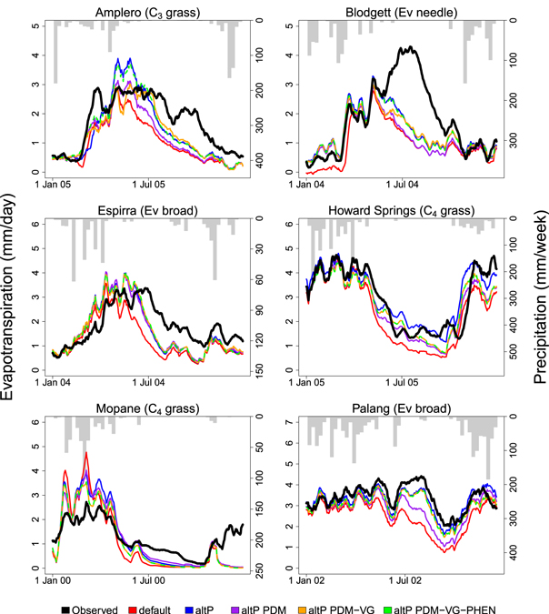
JULES-altP differed from the default version through a number of parameter changes and different process representations (see Best et al 2015). We examined the sensitivity of these changes to pinpoint the cause of the improved drought performance of JULES-altP (figure 3). The main changes responsible for the differences in the two versions of JULES, in order, were (a) switching off the representation of sub-grid scale heterogeneity in soil moisture, (b) switching the numerical solution for the soil hydraulics from Clapp and Hornberger (1978) to van Genuchten (1980) and (c) turning off the prognostic phenology scheme. The use of a sub-grid scale heterogeneity scheme for soil moisture (Moore 1985, Best et al 2011) is an attempt to represent horizontal site variations in soil moisture. Instead of representing soil moisture with a single uniform value across the grid cell, a probability distribution function is used. In theory this should allow the model to transition less abruptly into periods of drought as the surface has a more realistic representation of wet and dry regions (see Entekhabi and Eagleson 1989, Liang et al 1994). In reality, it appears that this scheme reduces deep soil water drainage due to increased surface runoff.
Figure 3. Evapotranspiration as observed and simulated by different configurations of JULES during an example one-year period. The time series show the 14 d running mean and run from January to December. The grey bars show 7 d precipitation totals. 'Default' and 'altP' are the default JULES-3.1 and JULES-altP models, respectively. 'PDM' and 'PHEN' are simulations with the probability distribution model and interactive phenology turned off, respectively. 'VG' is a simulation with the van Genuchten (1980) soil hydraulics scheme instead of the Clapp and Hornberger (1978) scheme.
Download figure:
Standard image High-resolution image
Changing the soil hydraulics from Clapp and Hornberger (1978) to van Genuchten (1980) explains the majority of the remaining differences in evaporation. However, if the change to the van Genuchten scheme is made whilst the sub-grid scale scheme is switched on, then in general the evaporation declines more rapidly than the original default JULES simulation during the drought periods, making the results worse. Hence we do not claim that the van Genuchten scheme performs better in JULES than the Clapp and Hornberger scheme, but that changes to the amount of water in the soil (through increased infiltration) and how this water hydraulically moves within the soil is important for an accurate solution. In the case of CABLE-GW, the choice of soil parameter values themselves has also been shown to be critical for accurate drought simulation (Ukkola et al 2016), highlighting the need to carefully treat soil hydraulic properties.
Finally, turning off the prognostic phenology scheme within JULES increases the evaporation in the early part of the growing season for two of the sites (Amplero and Tumbarumba). The phenology scheme does not develop the leaf area index (LAI) sufficiently in this part of the growing season to sustain the evaporation obtained when using a fixed default LAI value. However, the prognostic phenology gives evaporation that is in better agreement with the observations during the period of lower LAI values. This suggests that improvements in the results for the drought periods, from turning off the prognostic phenology, are not necessarily being achieved for the correct physical reasons.
Results from both the JULES and CABLE-GW models reinforce the conclusion that the way in which the soil hydrology is represented within models is critical for capturing the correct response in evaporation during sustained dry periods. LSMs have typically been developed to capture seasonal- to annual-scale hydrological processes and there is a clear need to better represent short-scale extreme phenomena, as well as to consider the uncertainty arising from soil hydraulic properties in the models.
4.2. Representation of plant water stress
CABLE-SLI includes alternative representations of soil hydrology, surface energy balance and plant water stress. Haverd et al (2016) separated the effects of these processes and demonstrated improvements to latent and sensible heat fluxes simulated by CABLE-SLI (relative to the default CABLE) at 19 globally distributed flux tower sites. These improvements were largely attributable to the alternative drought response function and the dampening effect of leaf litter on soil evaporation. Most LSMs (e.g. default CABLE and JULES, ORCHIDEE and CHTESSEL) limit gas exchange during drought following an empirical plant water stress function (β) (Verhoef and Egea 2014). Several limitations of this function have been noted. The implementation of the β function in models has generally been informed by limited or in some occasions, no experimental data (Medlyn et al 2016). It is also unclear how best to represent the effects of vertical variations in soil moisture on plant root water uptake for the calculation of β. De Kauwe et al (2015) showed that models which weight soil moisture content by root biomass (e.g. JULES, CABLE, COLASSiB and CLM) simulate a rapid depletion of soil water due to the models extracting soil water predominately from the top soil layers, which have a high root fraction, but relatively low absolute soil water content. The result of this weighting assumption is the rapid onset of drought typically observed in CABLE and many other LSMs in this study (figure 1).
CABLE-SLI uses an alternative approach for weighting the available soil water content used in its drought stress function. This scheme determines stomatal drought response using the soil water content of the wettest soil layer that has roots present and a drought response parameter, which controls the steepness of the drought response with respect to soil moisture (Haverd et al 2013). This is an attempt to capture the ecological optimality hypothesis that evolutionary selection pressures drive ecosystems towards maximal utilisation of available resources (Raupach 2005). This approach leads to improvements in simulations of ET at the onset of and during Edrought (figure 1). The drought response parameter could in theory be varied to account for variable drought responses amongst plant functional types, for which there is experimental evidence (McDowell et al 2008, Zhou et al 2013, 2014). However, in an assessment against 19 flux sites, while the optimum drought response parameter varied from site to site, there was no apparent relationship to aridity or plant functional type (Haverd et al 2016). In contrast, De Kauwe et al (2015) varied drought sensitivities from low in xeric (dry) ecosystems to high in mesic (humid) environments in CABLE-2.0 and showed the model to better capture observed ET during the 2003 European drought. Furthermore, the study identified the need to consider drought stress effects on both stomatal conductance and photosynthetic capacity in line with experimental evidence (Keenan et al 2009, Zhou et al 2013). Currently, LSMs differ in how they represent plant water stress, either reducing stomatal conductance or photosynthetic capacity or both (De Kauwe et al 2013) and consideration of both processes appears important (Keenan et al 2009, Egea et al 2011, Flexas et al 2012, Zhou et al 2013). PFT-specific drought responses may thus provide a further avenue for improving LSM simulations of drought.
4.3. Implications for other extremes
Previous studies have highlighted key differences among models when examining runoff metrics (Prudhomme et al 2011, Stahl et al 2011, Gudmundsson et al 2012, Tallaksen and Stahl 2014). In addition to errors in ET affecting soil moisture, errors in the hydraulic properties of the soil and the infiltration processes could both lead to differences in surface and sub-surface runoff. However, data were not available to evaluate these two runoff components from the models, and so we could not analyse them in this study. Clearly, future studies that evaluate all aspects of the terrestrial water cycle simultaneously would be ideal in order to examine these issues further.
There is another important implication of our results that is not immediately obvious. A key role of LSMs in climate models is to determine the partitioning of available energy into sensible and latent heat in interaction with the atmosphere. During water-stressed conditions, the latent heat flux is reduced and more available energy is exchanged as sensible heat. This land-atmosphere feedback has been shown to be important in the evolution of extreme temperatures including during the European heat wave of 2003 (Fischer et al 2007). Our results suggest that in site-scale offline simulations, LSMs systematically underestimate latent heat fluxes during water-stressed conditions and overestimate sensible heat flux at many sites (figure S3). This overestimation is greatest during periods of low rainfall and ET at many sites (see e.g. Amplero, Espirra and Palang during July), and is consistent with the finding by Haughton et al (2016) that partitioning was the largest source of error in LSMs' flux prediction in the PLUMBER experiment. These biases in sensible heat fluxes have the potential to affect the simulation of heat extremes, under the right synoptic conditions and cause an overestimation of heatwaves when these LSMs are running fully coupled.
5. Conclusions
Our results show that LSMs significantly overestimate the duration, magnitude and intensity of evaporative droughts (defined in this study as periods with low actual evapotranspiration and evaporative ratio) when evaluated against flux tower measurements of evapotranspiration. The 14 LSM versions analysed in this study overestimated annual Edrought duration by 12%–429% and Edrought magnitude by 10%–1484% across the six flux tower sites, pointing to large and systematic biases. Despite recent model improvements, the best performing model versions continue to over-predict annual Edrought duration by 12%–24%.
Many model development efforts concentrate on introducing new processes into LSMs. We suggest there is equally a need to re-examine existing model components in LSMs to improve simulations of water and heat fluxes during evaporative drought. A comparison of alternative model formulations demonstrated the importance of re-evaluating soil hydrological processes and water-plant interactions in LSMs, introducing mechanistic, data-driven parameterisations of fundamental land surface processes. Specifically, the representation of vertical soil water fluxes and plant water stress, together with a careful treatment of soil hydraulic properties, were shown to be important for determining evapotranspiration during water-stressed periods.
Most previous model evaluation studies have focussed on the mean state. Indeed, the hydrology in LSMs has been developed principally to capture longer-term mean behaviour. Our study has evaluated the capability of LSMs to capture the duration, magnitude and intensity of Edrought by focussing on periods where the observations point to the occurrence of low actual evapotranspiration. By focussing on more water-stressed periods, our study has identified a systematic bias in LSMs. We suggest therefore that there is an urgent need for more thorough evaluation of LSMs against extremes, for two associated reasons. First, this would enable the development of a better understanding of the limitations of current LSMs and inform how to re-parameterise important processes to improve the models. Second, this would enable improved projections of future changes in extremes. Since these include droughts and heatwaves, improvements would increase the value of LSMs and climate models in an area of direct societal need.
Acknowledgments
We acknowledge the support of the Australian Research Council Centre of Excellence for Climate System Science (CE110001028). MDK was supported by the Australian Research Council Linkage grant LP140100232. The contribution of VH was made possible by funding from the Australian Climate Change Science Program. We acknowledge the contribution of the PLUMBER participants for providing the LSM simulations used in this study. This work used eddy covariance data acquired by the FLUXNET community for the La Thuile FLUXNET release, supported by the following networks: AmeriFlux (US Department of Energy, Bio- logical and Environmental Research, Terrestrial Carbon Program (DE-FG02-04ER63917 and DE-FG02-04ER63911)), AfriFlux, AsiaFlux, CarboAfrica, CarboEuropeIP, CarboItaly, CarboMont, ChinaFlux, Fluxnet-Canada (supported by CFCAS, NSERC, BIOCAP, Environment Canada, and NRCan), GreenGrass, KoFlux, LBA, NECC, OzFlux, TCOS-Siberia, USCCC. We acknowledge the financial support to the eddy covariance data harmonisation provided by CarboEuropeIP, FAO-GTOS-TCO, iLEAPS, Max Planck Institute for Biogeochemistry, National Science Foundation, University of Tuscia, Université Laval and Environment Canada and US Department of Energy and the database development and technical support from Berkeley Water Center, Lawrence Berkeley National Laboratory, Microsoft Research eScience, Oak Ridge National Laboratory, University of California—Berkeley, University of Virginia. The data are available on request from the author (a.ukkola@unsw.edu.au).