

Abstract
Past studies suggest that forest fires contribute significantly to the formation of ozone in the troposphere. However, the emissions of ozone precursors from wildfires, and the mechanisms involved in ozone production from boreal fires, are very complicated. Moreover, an evaluation of the role of forest fires is prevented by the lack of direct observations of the ozone precursor, nitrogen oxides (NOx), and large uncertainties exist in the emissions inventories currently used for modelling. A comprehensive understanding of the important processes and factors involving wildfires has thus been unobtainable. We made 16 year consistent analyses of NOx emissions from boreal wildfires by using satellite observations of tropospheric nitrogen dioxides (NO2) from 1996 to 2011. We report substantial interannual variability of tropospheric NO2 originating from large boreal fires over Siberia in 1998, 2002, 2003, 2006, and 2008; and over Alaska in 2004, 2005, and 2009. Monthly comparisons of NO2 enhancements with fire radiative power (FRP) show reasonably strong correlation, suggesting that FRP is a better proxy than burned area for boreal fire NOx emissions. We provide space-based constraints on NOx emission factors (EFs) for Siberian and Alaskan fires. Although the associated uncertainty is relatively large, the derived EFs fall into a in reasonably agreeable range with those previously determined by in situ ground-based and airborne observations over these regions.
Export citation and abstract BibTeX RIS

Content from this work may be used under the terms of the Creative Commons Attribution 3.0 licence. Any further distribution of this work must maintain attribution to the author(s) and the title of the work, journal citation and DOI.
1. Introduction
Biomass burning plays an important role in the Earth's climate system and global biogeochemical cycles, and wildfires in boreal regions such as Siberia and Alaska are important sources of trace gases and aerosols emitted into the atmosphere. In the atmosphere, nitrogen oxides (NOx) and non-methane volatile organic compounds (NMVOCs) emitted from fires are subject to photochemical oxidation, affecting the oxidizing capacity and radiative budget of the atmosphere by serving as precursors of tropospheric ozone (O3). Although it is generally believed that biomass burning is a substantial contributor to tropospheric O3 production, observational evidence during the past decades has shown contradicting pictures, suggesting that the emissions of O3 precursors from wildfires, and the mechanisms involved in O3 production from boreal fires, are very complicated and nonlinear. For example, plume chemistry is not often resolved, injection height is often not known, and chemical interference of the emitted gases with aerosols in the plume can alter photolysis rates and provide heterogeneous surfaces.
The emission and long-range transport of carbon monoxide (CO) from fires has been well studied, both in terms of pollution episodes and interannual variability (e.g., Tanimoto et al 2000, 2009, Yurganov et al 2004, 2005, 2010, Turquety et al 2007). The enhancement of CO from fire emissions is identifiable due to its relatively long lifetime, and it is known that Siberian and Alaskan fires contribute substantially to the global CO budget (van der Werf et al 2010, van Leeuwen and van der Werf 2011). However, in contrast to CO, the impact from boreal fires on O3 has been less well quantified, in spite of its potentially important role in controlling day-to-day variations, interannual variability, and long-term trends of tropospheric O3.
The episodic enhancement of O3 relative to CO in boreal fire plumes has been examined in several observations, with diverse results ranging from negative to positive O3 production (e.g., Tanimoto et al 2000, 2008, Jaffe et al 2004). The magnitude of O3 enhancement in biomass burning plumes is a recent topic of discussion (Jaffe and Wigder 2012). Identifying the impact on O3 interannual variability is also challenging, as it is only in the range of 0–5 ppbv (Tanimoto 2009). Thus, investigations relating to tropospheric O3 are considerably more complicated than those pertaining to CO, because O3 production depends on various factors including fire emissions, photochemical reactions, meteorology, and aerosol effects.
One of the major constraints to O3 production is the availability of NOx emitted from primary sources, as NOx is a key precursor for O3 production. However, the levels, variability, and distribution of NOx near fire regions have not been extensively examined, because measurements are generally not conducted near fires, and measurements made at remote downwind sites are of limited use due to the short lifetime of NOx. In addition, measurements of NOx are not widely available from operational monitoring networks. Thus, the understanding of NOx emissions from fires has been limited. Investigations using satellite NO2 observations to analyse changes in NOx emissions have been reported for a variety of emission sources, mainly from anthropogenic sources (e.g., Ghude et al 2008, Castellanos and Boersma 2012, Miyazaki et al 2012) and from soil (Ghude et al 2010, Hudman et al 2010). Several studies have recently explored biomass burning sources, including wildfires in Western North America (Mebust et al 2011), in Western Siberia near Moscow in 2010 (Huijnen et al 2012), and in South America (Castellanos et al 2014), and these studies have focused on the contribution of relatively intensive burning to emissions of NOx. In addition, global-scale biomass burning emissions of NOx from steadily burning areas have very recently been reported in terms of climatological emissions, for 2005–2011 using an Ozone Monitoring Instrument (OMI) (Mebust and Cohen 2014) and for 2007–2011 using the Global Ozone Monitoring Experiment-2 (GOME-2) and OMI sensors (Schreier et al 2014). However, detailed information, such as seasonal and interannual variability, has not yet been studied, especially not on the 16 year timescale as done here. In particular, the variability of NOx emissions due to wildfires in boreal regions has not been examined, even though it is expected to be substantial.
In general, interannual variability in tropospheric NO2 columns is small compared to multi-year trends driven by anthropogenic emissions (e.g., Richter et al 2005, Van der A et al 2008, Hilboll et al 2013). In this study, we examined polar-orbiting satellite NO2 observations over boreal forests, where data to constrain biomass burning emissions has been lacking relative to other ecological regions, while the contribution of fires to atmospheric chemistry is likely larger due to sparse population, and the sensitivity to climate change is higher relative to mid-latitude ecosystems. We found that satellite instruments are capable of detecting interannual variability of tropospheric NO2 over Siberia and Alaska for the period 1996–2011. Enhancements noted therein were attributed to NOx emissions from forest fires. A systematic examination of the NOx emission coefficient due to wildfires was then conducted, with a particular emphasis on the years with strong fire activity (hereafter referred to as 'large-fire years') of 2002, 2003, 2006, and 2008 for Siberia; and 2004, 2005, and 2009 for Alaska. Analysis of tropospheric NO2 enhancements with fire radiative power (FRP) revealed reasonable correlations, suggesting that fire energy is a good proxy for NOx emissions from boreal fires.
2. Satellite observations and emissions inventory
We used robust and consistent long-term records of polar-orbital satellite data from the GOME and SCanning Imaging Absorption spectroMeter for Atmospheric CartograpHY (SCIAMACHY) sensors on-board the ERS-2 and Envisat platforms, respectively. Both spectrometers are nadir-viewing, measuring backscattered light from the Earth's atmosphere in the ultraviolet and visible wavelength range. The GOME observations provide a ground pixel size of 40 × 320 km2 and equatorial overpasses at 10:30 LT. Data are available since 1995, with global coverage every 3 days. SCIAMACHY has been observing the atmosphere since 2002, in alternating limb and nadir directions, and nadir observations only are used for tropospheric NO2 retrieval, resulting in global coverage every 6 days. Data frequency is improved at high latitudes. For example, it takes 2–3 days to achieve complete coverage at 60°N. The SCIAMACHY observations provide a ground pixel size of 30 × 60 km2, and an equatorial overpass time at 10:00 LT. The updated product of the retrieval algorithm (version 2.0) was used, and is publicly available on the TEMIS project website (www.temis.nl). This product was evaluated for detailed error estimates and kernel information, as reported in Boersma et al (2004, 2011). Only observations with a top-of-atmosphere radiance fraction of less than 50% from clouds (and aerosols) were used. We used the monthly means of tropospheric NO2 column data with a horizontal resolution of 0.25° × 0.25° from 1996 to 2011. Daily satellite data have been interpolated onto a 0.25° × 0.25° grid with the individual pixel's fractional coverage of the grid cell as a weight in the subsequent calculation of the monthly average. GOME and SCIAMACHY data overlapped for the period from August 2002 to June 2003. For a detailed comparison to FRP, the 0.25° × 0.25° data set was re-gridded to a 1° × 1° resolution.
We also used satellite data from the MODerate resolution Imaging Spectroradiometers (MODIS) on board NASA's Terra satellite launched in December 1999, which have corresponding equatorial overpass times of 10:30 LT. MODIS data from the Aqua satellite was not utilized because the overpass time is 13:30 LT, which does not match with GOME or SCIAMACHY, and data is not available before 2002. The MODIS instrument has 36 spectral bands ranging in wavelength from 0.4 to 14.4 μm. Differences in 4 and 11 μm black body radiation emitted at combustion temperatures were used to locate active fires at a horizontal resolution of 1 km2. The 'MOD14CM1.005' product was also used, which is available at a horizontal resolution of 1° × 1°, to examine FRP as a proxy of the radiant component of energy release from fires (Kaufman et al 1998, Justice et al 2002).
The third satellite-based product used was the Global Fire Emissions database (GFED), which relies on improved MODIS-derived estimates of areas burned (or burned scars), fire activity, and plant productivity, and a revised version of the Carnegie–Ames–Stanford-Approach biogeochemical model. To calculate emissions of trace gases and aerosols, emission factors (EFs) were applied based on the studies of Andreae and Merlet (2001) or Akagi et al (2011). The GFED version 3 data set, with a horizontal resolution of 0.5° × 0.5°, has been available since 1997 (http://globalfiredata.org/). Updates from version 2 include improved satellite input data, explicitly accounting for deforestation and forest degradation fires in the model, partitioning fire emissions into different source categories, and adding an uncertainty analysis (van der Werf et al 2010). Monthly data re-gridded to a 1° × 1° resolution was used to match with the horizontal resolution of FRP.
3. Results
A systematic examination of boreal fires occurring in Siberia and Alaska was made for the period 1996–2011. Figure 1 shows the 15 year time series of regional mean NOx emissions as calculated by GFEDv3 and FRP, for Siberia and Alaska, throughout the period 1996–2011. We focused on the regions of Eastern Siberia (48–65°N, 98–142°E) and the entire area of Alaska (60–70°N, 160–120°W) to eliminate possible influences from anthropogenic NOx emissions in more densely populated areas in Western and Central Siberia, and in Canada. GFEDv3 predicted large NOx emissions from Siberian fires in 1998, 2002, 2003, 2006, and 2008, while the emissions were also significant in other years during the spring–summer seasons (April–October). This was in accordance with previous papers reporting the emissions of trace gases and aerosols from Siberian fires (Yurganov et al 2010). The time-series of FRP shows clear seasonal cycles from the year 2001. Similar to the results from GFEDv3, the seasonality of FRP indicates burning in warm seasons in spring and summer, but also extends to cold seasons; results yield broader peaks than GFEDv3. The interannual variability of the magnitude of FRP is generally similar to that of GFEDv3; for example, high FRP is indicated in 2003 and 2008. However, the contrast between large-fire years and small-fire years is not as large as that of GFEDv3.
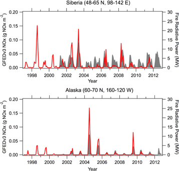
Figure 1. Fifteen year time series (1996–2011) of regional mean NOx emissions calculated by GFEDv3 (red lines, left axis), and fire radiative power (grey areas, right axis) for Siberia (48–65°N, 98–142°E) and Alaska (60–70°N, 160–120°W).
Download figure:
Standard image High-resolution imageFor Alaska, GFEDv3 predicts large NOx emissions from fires in 2004, 2005, and 2009, but considerably less emissions in other years during summer seasons (May–August). The burning period in Alaska is much shorter than that of Siberia. Emissions of trace gases and aerosols from Alaskan fires in these years have been previously reported (Turquety et al 2007). The time-series of FRP shows clear seasonal cycles, and indicates high FRP in 2004, 2005, and 2009. It is interesting to note that the agreement between FRP and GFEDv3 is much better for Alaska than for Siberia, and the burning period predicted by FRP is the same that of GFEDv3. Overall, the seasonal and interannual contrasts between large-fire years and small-fire years are in good agreement. In this analysis, we focus on the large-fire years of 2002, 2003, 2006, and 2008 for Siberia; and 2004, 2005, and 2009 for Alaska.
The seasonality of 'baseline' tropospheric NO2 columns over Siberia and Alaska was examined by calculating the climatological means from small-fire years. For Siberia, we calculated the 11 year climatology from 1996, 1997, 1999, 2000, 2001, 2004, 2005, 2007, 2009, 2010, and 2011, when fire events were minor relative to the large-fire years of 1998, 2002, 2003, 2006, and 2008. Similarly, for Alaska, we calculated the 13 year climatology from 1996, 1997, 1998, 1999, 2000, 2001, 2002, 2003, 2006, 2007, 2008, 2010, and 2011. Wintertime data (from December to March) for Alaska were neglected because of the insufficient amount of data (less than 1000 pixels) available over high latitudes in boreal winter due to no light. Regional mean tropospheric NO2 columns over Siberia were in the range from 0.6 to 1.2 × 10¹⁵ molecules cm–2 over the course of year, and were associated with substantial seasonal variations, showing a summer minimum and winter maximum, reflecting the varying lifetime of NO2 in the troposphere. The levels of baseline mean tropospheric NO2 columns over Alaska in summer were in the range of 0.4–0.6 × 10¹⁵ molecules cm–2, which was slightly lower than, but close to, those over Siberia in summer. The levels in other months were lower than over Siberia, resulting in overall negligible seasonal features.
The levels of tropospheric NO2 columns over these boreal regions were low, making the detection of the NO2 enhancement due to boreal fires challenging. In order to better detect and analyse the enhancements of tropospheric NO2 columns due to boreal fires, we derived monthly anomalies for Siberia and Alaska by subtracting baseline seasonal cycles as described above. Figure 2 shows interannual variability of the regional-mean enhancement of the tropospheric NO2 column beyond baseline levels over Siberia and Alaska, for the period 1996–2011. The enhancements are seen to be subtle, but visible, in large-fire years during the summer of 2002, and during the springs of 2003 and 2006 for Siberia. Similarly, enhancements are visible in large-fire years in the summers of 2004, 2005, and 2009 for Alaska.
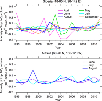
Figure 2. Interannual variability in the regional-mean enhancement of the tropospheric NO2 column beyond baseline levels over Siberia and Alaska for the period 1996–2011.
Download figure:
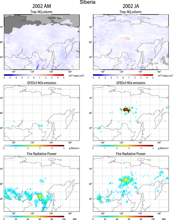
Standard image High-resolution imageFigure 3 illustrates the geographical distribution of enhancements of the tropospheric NO2 column, NOx emissions estimated by GFEDv3, and mean FRP as detected by MODIS over Siberia for 2002, 2003, 2006, and 2008; and over Alaska for 2004, 2005, and 2009. The NO2 enhancements and mean FRP are temporally averaged, while GFEDv3 NOx emissions are totalled over the burning seasons for Siberia and Alaska. While relatively weak in magnitude (on the order of 1015 molecules cm–2), significant hot spots of the tropospheric NO2 enhancements are evident, and the location and intensity of NO2 enhancements vary depending on the burning event. Fires often occurred East of Lake Baikal in the latitudinal zone of 50–65°N, in far Eastern Siberia. In Alaska, although the horizontal scale of the fires was small compared to Siberia, the NO2 enhancements can still be seen from GOME and SCIAMACHY retrievals.
Download figure:
Standard image High-resolution image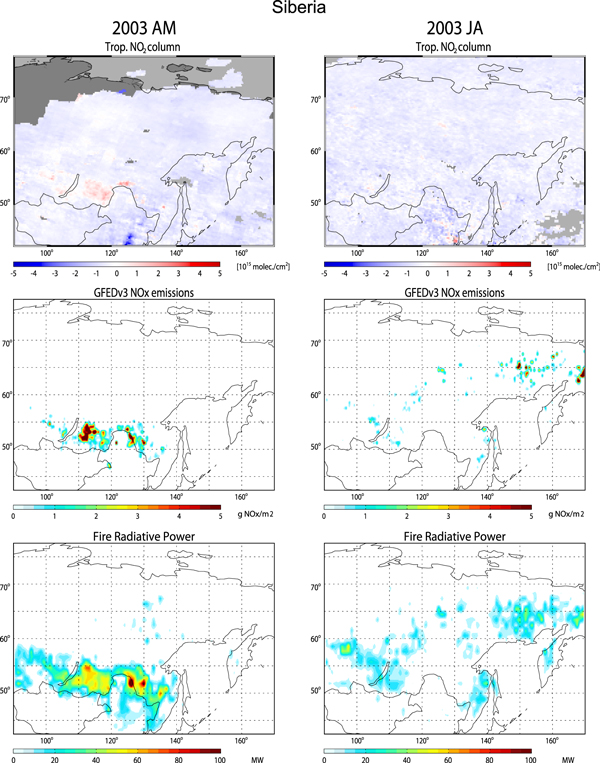
Download figure:
Standard image High-resolution image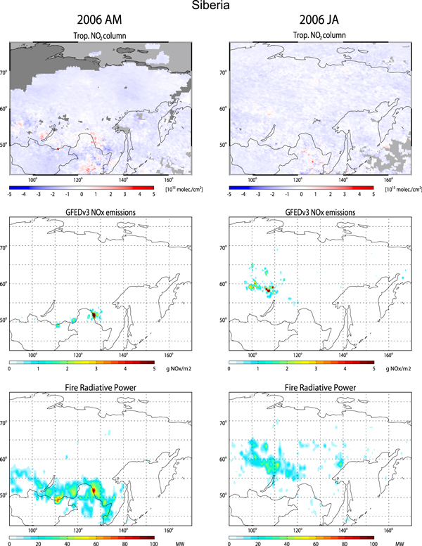
Download figure:
Standard image High-resolution image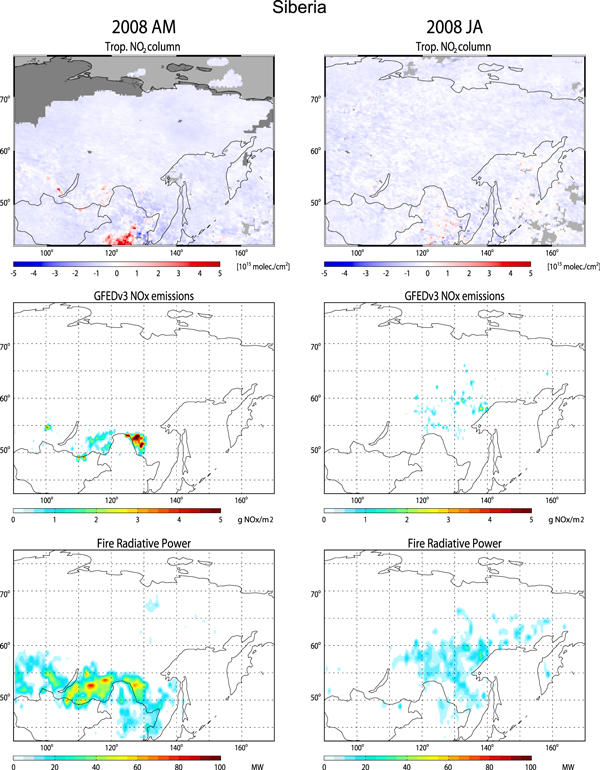
Download figure:
Standard image High-resolution image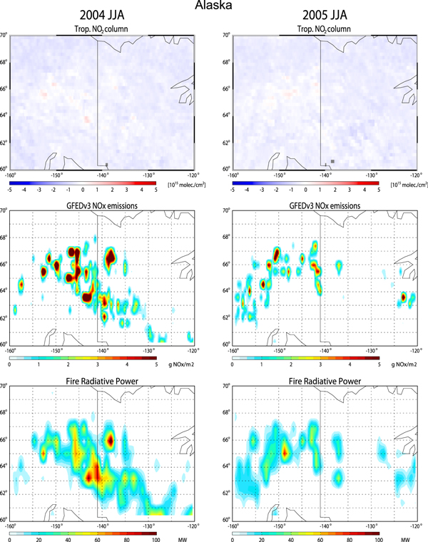
Download figure:
Standard image High-resolution image
Figure 3. Enhancements of tropospheric NO2 column (upper panel), NOx emissions estimated by GFEDv3 (middle panel), and mean FRP (bottom panel) detected by MODIS over Siberia for 2002, 2003, 2006, and 2008; and over Alaska for 2004, 2005, and 2009. AM, JA, and JJA denote April–May, July–August, and June–July–August, respectively.
Download figure:
Standard image High-resolution imageFor both Siberia and Alaska, locations of NO2 enhancements are in clear correspondence to those predicted by GFEDv3 and FRP, suggesting that enhancements are attributed to NOx emissions from forest fires in Siberia and Alaska. It is interesting to note from a comparison of GFEDv3 estimates with FRP detections, that there are slight but substantial differences in the location and relative magnitude between these two parameters. For example, in April/May of 2008, GFEDv3 predicted strong emissions around the border between Russia and Mongolia (50–55°N, 120–130°E). So did FRP, but it indicated comparably strong burnings in the West (50–55°N, 110–120°E). In general, the fires indicated by mean FRP cover a large domain than those estimated from GFEDv3. GFEDv3 missed the emissions in Eastern Siberia. The geographical distributions of GFEDv3 emissions rely on the burned area retrieved from MODIS. Hence, these differences would basically reflect the differences between burned scars and FRP.
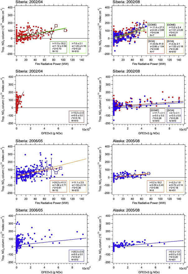
In order to explore quantitative correspondence of the NO2 enhancements with GFEDv3 estimates and FRP observations, we examined 1° × 1° grid correlations of the NO2 enhancements against GFEDv3 NOx emissions and FRP data on a monthly basis. Figure 4 shows examples of the correlations of NO2 enhancements with FRP and GFEDv3 for Siberia in 2002 and 2006, and for Alaska in 2005. Although the plots are scattered owing to weak satellite signals, we can see a certain degree of correlation with FRP and GFEDv3, but correlations are much better between the satellite NO2 retrievals and FRP. For example, in April 2002, GFEDv3 predicts negligible NOx emissions, but FRP shows a relatively good correlation with NO2 enhancements. In general, NO2 enhancements show a better correlative behaviour with FRP than GFEDv3, suggesting that FRP is a better proxy than burned area for NOx emissions from boreal fires. This is reasonable since FRP is thought to be a diagnostic for high-temperature flaming combustion, which oxidizes nitrogen more effectively.
Figure 4. Examples of correlations of tropospheric NO2 column enhancements with mean FRP observed by MODIS and NOx emissions estimates by GFEDv3, for Siberia and Alaska.
Download figure:
Standard image High-resolution image
Slopes and determination coefficients (r2) were calculated for all the 1° × 1° data, and for 10 Mega Watt (MW)-binned data for correlations of tropospheric NO2 enhancement with FRP. Although in many months the correlations were not statistically significant due to weak signals, statistically significant slopes were found (as indicated by bold numbers in the grey-hatched cells) in 16 out of 66 months for Siberia, and 3 months out of 33 months for Alaska. (Tables S1 and S2 summarize the monthly-based statistics of tropospheric NO2 enhancement correlations with FRP, for Siberian and Alaskan fires, respectively.) The slopes of tropospheric NO2 enhancement correlations to FRP are regarded as the enhancement ratio (ER) of the tropospheric NO2 column due to forest fires (i.e., ΔNO2 column/ΔFRP). By using the ER, the mass emission coefficient (MEC) of NOx emitted from boreal fires can be calculated, following the method devised by the University of Bremen (Schreier et al 2014) that converts the NO2 column number density (in molecules cm−2) as retrieved from satellite instruments, into the column mass concentration (in g cm−2), with the help of Avogadro's number (NA, molecules mol−1), the molar mass (M) of NO (30 g mol−1), and the 1° × 1° grid area (in cm2), and by assuming a NO2/NOx ratio of 0.75 and a lifetime of NOx (in seconds), which we assume to be in the range from 21600 s (6 h) to 7200 s (2 h). The resulting MEC is in the unit of g NOx (as NO) MW−1 s−1, (or g NOx (as NO) MJ−1), because the emissions of NOx are reported as NO in the emission inventories for a later comparison. In the calculation of the MEC, the ER was used only when: (1) the slopes for both the all- and binned-data were statistically significant; and (2) the determination coefficients (r2) for binned-data were greater than 0.4. Thresholds for determination coefficients, based on all-data, were relaxed to 0.3 and 0.1 for Siberia and Alaska, respectively, to allow reasonable data selection.
Along with two previous studies by Mebust and Cohen (2014) and Schreier et al (2014), the present work examines the relationship of satellite-derived tropospheric NO2 with FRP, built upon the method first reported for the study of aerosol by Ichoku and Kaufman (2005). Hence, these three studies all apply the same principle, but with minor differences in data and technical processing. The differences include satellite sensors employed (and overpass times), temporal/spatial resolution of the data used, definition of background signals, and NOx lifetime assumed. We relied on the satellite observations by GOME and SCIAMACHY, while Mebust and Cohen (2014) relied on those by OMI and Schreier et al (2014) used those by both OMI and GOME-2. The local time of the GOME, SCIAMACHY, and GOME-2 observations is in the morning, while that of the OMI observations is in the early afternoon. Schreier et al (2014) and we used monthly-mean, 1° × 1° gridded data, while Mebust and Cohen (2014) used individual pixels observed by the satellite. The definition of the background NO2 level is rather different. We used climatological values based on monthly data in low-fire years, and did not use the intercepts from the regressions in figure 4, Mebust and Cohen (2014) used fire-free data at the same location within the a 120 day time window, and Schreier et al (2014) used intercepts of the linear regression lines for the regional NO2-versus-FRP correlations based on monthly data. For the lifetime of NOx, we used both 2 and 6 h, as lower and upper limits, respectively, while Schreier et al (2014) used for the monthly data a 6 h lifetime based on Beirle et al (2011) who examined NOx plumes from the megacities, and Mebust and Cohen (2014) chose 2 h based on a quoted range of lifetimes between 2–3 and 7 h from past observations of fire plumes (Yokelson et al 1999, Alvarado et al 2010). We argue that the NOx lifetime could vary from individual fire plumes to monthly averaged fields, with the overall lifetime possibly being longer in monthly fields than in fire plumes. Instantaneous NO2 lifetimes are generally longer in the morning (e.g, the overpass time at 10:00) than in the afternoon (e.g., the overpass time at 14:30), when chemical regimes are more conducive to fast NO2 oxidation due to higher temperatures, more dilution, stronger photochemistry. Oxidation chemistry in forest fire plumes can be different from in megacity plumes, and boreal fires occur more often during the summer when photochemistry is faster than in winter. With all these discussions being considered, we conclude that the accuracy of the lifetime assumption is not sufficiently well established yet, and treat a range of possibilities from 2 to 6 h to be equal and as an uncertainty range.
4. Discussion
Table 1 shows a summary of the ER and MEC for Siberia and Alaska. For calculations, data with robust statistical significance (as shown with a bold font in grey-hatched cells in tables S1 and S2) were used. For Siberia, the ER was calculated as 1.58 ± 1.09 × 10¹³ molecules cm−2 MW−1 (N = 17 months) and 1.15 ± 0.51 × 10¹³ molecules cm−2 MW−1 (N = 17 months), for binned- and all- 1° × 1° data, respectively; leading to 1.37 ± 0.80 × 10¹³ molecules cm−2 MW−1 (N = 34 months). Determination of the ER for Alaska was more difficult due to the reduced amount of statistically significant data available. Nevertheless, it was calculated as 0.53 ± 0.05 × 10¹³ molecules cm−2 MW−1 (N = 3 months) and 0.59 ± 0.18 × 10¹³ molecules cm−2 MW−1 (N = 3 months) for binned- and all- 1° × 1° data, respectively, resulting in 0.56 ± 0.12 × 10¹³ molecules cm−2 MW−1 (N = 6 months). The resulting MECs were calculated as 4.21 ± 2.47 for 6 h lifetime (or 12.62 ± 7.40 for 2 h lifetime) and 1.73 ± 0.36 for 6 h lifetime (or 5.18 ± 1.07 for 2 h lifetime) g NOx MJ−1 (as NO) for Siberia and Alaska, respectively. Although within the range of uncertainty, there was a difference of a factor of 2 in the mean MECs between Siberia and Alaska.
Table 1. NO2 enhancement ratio, NOx mass emission coefficient, and NOx emission factor for Siberian and Alaskan fires.
| Siberia | Alaska | ||||
|---|---|---|---|---|---|
| Region | Binned data (r2 > 0.4) | All data (r2 > 0.3) | Binned data (r2 > 0.4) | All data (r2 > 0.1) | |
| NO2 enhancement ratio (1013 molecules cm−2 MW−1) | 1.58 ± 1.09 (N = 17) | 1.15 ± 0.51 (N = 17) | 0.53 ± 0.05 (N = 3) | 0.59 ± 0.18 (N = 3) | |
| Average | 1.37 ± 0.80 (N = 34) | 0.56 ± 0.12 (N = 6) | |||
| NOx mass emission coefficient (g NOx MJ−1 as NO) | 4.21 ± 2.47 (6 h lifetime) | 1.73 ± 0.36 (6 h lifetime) | |||
| 12.62 ± 7.40 (2 h lifetime) | 5.18 ± 1.07 (2 h lifetime) | ||||
| NOx emission factor (g kg−1 as NO) | This work | 2.71 ± 1.59 (6 h lifetime) | 1.11 ± 0.23 (6 h lifetime) | ||
| 8.14 ± 4.78 (2 h lifetime) | 3.34 ± 0.69 (2 h lifetime) | ||||
| Akagi et al (2011) | 0.90 ± 0.69 (for boreal forest); 1.12 ± 0.69 (for extratropical forest) | ||||
| Andreae and Merlet (2001) | 3.0 ± 1.4 (for extratropical forest) | ||||
4.1. Comparison of MEC
By using OMI-derived NO2 data, Mebust and Cohen (2014) determined the MEC of NOx from the burning of biomass including that of boreal forest, and by assuming a NOx lifetime of 2 h the MEC for boreal fires was calculated as 0.250 ± 0.033 g NOx MJ−1. They also noted that the MECs were similar in different ecosystem regions regardless of biomes, and were in the range of 0.250–0.362 g NOx MJ−1. In contrast, Schreier et al (2014) used monthly data from both OMI and GOME-2 observations, assumed a lifetime of 6 h, and reported that MECs varied within a range of 0.28–1.56 g NOx MJ−1 depending on vegetation types. However, boreal forest was not included in that analysis. Therefore, substantial discrepancies exist between past satellite-based studies, and these are likely related to the inherently varying lifetimes of NOx in individual fire plumes, the diurnal variability of emissions, and the chemical transformation of NOx.
As mentioned above, there are some differences among the three approaches. If the large-fire years resulted in higher background levels than the small-fire years that we adopted as the background, this could be a possible source of uncertainty. However, since the differences in the background levels between large- and small-fire years were usually negligible (within ±10%, at most), this does not constitute a source of error. As seen above, differences by a factor of 3 in the NOx lifetime assumption (6 versus 2 h) can greatly affect the MEC estimates. Another source of the uncertainty is the use of monthly data that involves a number of averaging steps, resulting in weak relationships between the FRP and tropospheric NO2, compared to the correlations on a daily basis.
The values of MECs reported in this study, of 1.7–4.2 (with 6 h lifetime) and 5.2–12.6 (with 2 h lifetime) g NOx MJ−1, appear high compared to those in the previous two studies. However, past studies yielded climatological MECs, and we used large-fire data (data with robust statistical significance, even for monthly means, as shown in tables S1 and S2), which would result in higher values. It is understood that there is a natural variability in the values of MECs, depending on burning, climate, and fuel conditions in individual fires, and the MECs observed in this study seem within a reasonable range of this natural variability. In order to obtain rough estimates of 'climatological' MECs by our approach, we considered all the monthly-based statistics from the tropospheric NO2-versus-FRP correlations (regardless of statistical significance in tables S1 and S2). The calculated 'climatological' MECs fell into the range of 0.4–1.7 (with 6 h lifetime) and 1.2–4.9 (with 2 h lifetime) g NOx MJ−1 as NO. We see an improved agreement, in particular with Schreier et al (2014) who provided climatological estimates by using monthly data with the assumption of a 6 h lifetime. It seems that this can explain a substantial portion (60–80%) of the discrepancy between our work and past estimates.
4.2. Comparison of EFs
In this section, we derive EF from the MEC, make a comparison with previous estimates, and discuss the degree of agreement. Previous efforts to determine EFs, based on in situ observations and burning experiments, are well summarized in the comprehensive reviews of Andreae and Merlet (2001) and Akagi et al (2011). It should be noted that, for some species from some sources, EFs are calculated based only on a handful of available measurements; hence, the reported EFs are not necessarily robust and need to be continuously evaluated. For example in Akagi et al (2011), the EF of NOx from boreal fires was calculated from one ground-based measurement and three airborne measurements in North America. It should also be noted that the EFs for boreal fires in these reviews are biased to North American fires, since the raw data was mostly collected in North America. Furthermore, EFs can greatly vary depending on the burning conditions (flaming to smoldering), availability of air and humidity, and the type of fuel involved. For example, emissions of CO2 and NOx are predominant in flaming conditions, while those of CO and NMVOCs predominate in smoldering. For short-lived species including NOx, the age of air samples observed is also important in determination of EFs, as demonstrated by Kudo et al (2014) who showed the rapid loss of alkenes in fire plumes even within a few hours. Without appropriate correction by air mass age therefore, EFs would be greatly underestimated.
In order to convert MECs to EFs, a conversion factor (CF) from FRP to dry biomass burned is required. Based on ground-based experiments linking direct FRP observations to biomass consumption for small-scale fires, Wooster et al (2005) proposed a universal CF of 0.368 kg MJ−1 for the conversion from FRP to dry matter burned. A similar value of 0.41 kg MJ−1 was proposed by Vermote et al (2009). In a comparison of the dry matter combustion rate of FRP and GFEDv3, Heil et al (2010) found that the FRP-dry matter burned CF depended on the land cover type. Kaiser et al (2012) determined land-cover dependent CF for eight land cover classes, where the CF for boreal fires (extratropical forest with organic soil by their definition) was 1.55 kg MJ−1. Therefore, in recognition that there is a substantial range (approximately ± 60%) in CF estimates, we adopt the CF of 1.55 kg MJ−1 from Kaiser et al (2012) to calculate the EFs in our analysis, since boreal forest has a huge pool of biomass at ground-level or below-ground (e.g., peat) which is a major source of fuel (not the leaves and trunk). The resulting EFs for Siberian and Alaskan fires are therefore 2.71 ± 1.59 and 1.11 ± 0.23 g kg−1, respectively, for the NOx lifetime of 6 h. For the NOx lifetime of 2 h, the EFs are 8.14 ± 4.78 and 3.34 ± 0.69 g kg−1, respectively. Possible explanation would be higher fire intensity (e.g., more flaming) and/or more availability of peat-like biomass in Siberia than Alaska.
Akagi et al (2011) reported the EF of NOx explicitly for boreal forest fires as 0.90 ± 0.69 g NOx kg−1 dry biomass as NO. Alvarado et al (2010) derived an NOx EF of 1.06 g NOx kg−1 dry biomass for Canadian fire plumes. Andreae and Merlet (2001) reported EFs of NOx for extratropical forest fires as 3.0 ± 1.4 g NOx kg−1. Since extratropical forest is comprised of boreal and temperate forest, Akagi et al (2011) gave a greater weight to boreal forest fire EF than temperate forest fire EF (2.51 ± 1.02), with a ratio of 87:13 (based on relative global fuel consumption), to generate their extratropical EF of 1.12 ± 0.69 g NOx kg−1. Hence, at a maximum there is roughly a factor difference of 3 between these two inventories. Akagi et al (2011) noted that their total EFs for boreal fires reflected a large component of smoldering combustion data, suggesting that the EF of NOx for boreal fires was dominantly calculated by smoldering burning, which releases much less NOx emissions than flaming burning. Smoldering is not always dominant as there is evidence of pyro-convective fires over boreal forest (Fromm and Servranckx 2003). Therefore, the true EF of NOx from boreal fires would be in the range of 1–3 g NOx kg−1, and the above-derived satellite-based values of 1.1–8.1 partly overlap with this range. While the advantage of satellite-based analysis is that it enables statistical robustness due to the huge number of data, the associated uncertainty is high compared to in situ measurements used to determine EFs in the previous reviews. It is therefore considered that both in situ measurement- and satellite-based approaches should be used in tandem to further test our understanding of EFs, and to narrow down the uncertainty of estimates.
Acknowledgments
We thank Krishna P Vadrevu for valuable discussion on fire intensity, and Kimiko Suto, Haruka Yamagishi, and Edit Nagy-Tanaka for technical support. We acknowledge the tropospheric NO2 column data from the GOME and SCIAMACHY sensors available at www.temis.nl. We also thank NASA for providing MODIS fire radiative power data. The Giovanni online data system, developed and maintained by NASA GES DISC, was utilized. Data of GFED were obtained at http://globalfiredata.org. This work was supported by the Environmental Research and Technology Development Fund (2-1505) of the Ministry of the Environment, Japan. The authors thank three reviewers for their comments for improving the paper.