


Abstract
The interannual variability in the Baltic Sea ice cover is strongly influenced by large scale atmospheric circulation. Recent progress in forecasting of the winter North Atlantic Oscillation (NAO) provides the possibility of skilful seasonal predictions of Baltic Sea ice conditions. In this paper we use a state-of-the-art forecast system to assess the predictability of the Baltic Sea annual maximum ice extent (MIE). We find a useful level of skill in retrospective forecasts initialized as early as the beginning of November. The forecast system can explain as much as 30% of the observed variability in MIE over the period 1993–2012. This skill is derived from the predictability of the NAO by using statistical relationships between the NAO and MIE in observations, while explicit simulations of sea ice have a less predictive skill. This result supports the idea that the NAO represents the main source of seasonal predictability for Northern Europe.
Export citation and abstract BibTeX RIS

Content from this work may be used under the terms of the Creative Commons Attribution 3.0 licence. Any further distribution of this work must maintain attribution to the author(s) and the title of the work, journal citation and DOI.
Introduction
Each winter navigation in the Baltic Sea is restricted by ice cover. Ice season lasts for 3–6 months making shipping in the ice covered areas dependent on ice-breakers (Vihma and Haapala 2009). During the severest of winters ice can cover the whole Baltic Sea area of 422 000 km2, although the last time these conditions were observed was in the winter of 1946/47, more than a half century ago. During mild winters the ice cover is restricted to the Gulf of Bothnia, the Gulf of Finland and the Gulf of Riga. The smallest annual maximum of ice extent of 49 000 km2 was observed in 2007/08 (Luomaranta et al 2014). Between these two extremes the ice cover has a strong interannual variability, which has a great influence on the economics of the region (Juga et al 2012). For example, ice-breaker costs during the severe ice winter of 2010/2011, when maximum ice extent was 309 000 km2, reached 45 million euros, more than six times larger than during the mild winter of 2007/08 (Baltic Icebreaking Management 2008, 2011). The need to better prepare for such expense calls for skilful seasonal forecasts of Baltic Sea ice conditions.
Many previous studies (Koslowski and Loewe 1994, Tinz 1996, Omstedt and Chen 2001, Jevrejeva et al 2003) have shown that interannual variability of the Baltic Sea seasonal ice cover is strongly influenced by atmospheric circulation variability associated with the North Atlantic Oscillation (NAO). Indeed, the NAO was positive during the smallest sea ice extent year of 2007/8 and negative during the severe ice winter of 2010/11 (Maidens et al 2013). In particular, Tinz (1996) showed that a zonal index, closely related to the NAO, could explain 54% of interannual variability in the annual maximum sea ice extent (MIE) during the period 1899–1993. Recently, Scaife et al (2014) reported skilful forecasts of the winter mean NAO index and showed that this skill translates into skilful predictions of European winter climate. The purpose of our paper is to document whether this can lead to skilful predictions of Baltic Sea MIE using output from the same forecast system.
Data
We use historical forecasts (hindcasts) for the twenty winters from 1992/93 to 2011/12 produced by the Met Office Global Seasonal forecast System 5 (GloSea5), the same data set which was used in and described by Scaife et al (2014). The GloSea5 forecast system is fully documented in MacLachlan et al (2014). Briefly, the system is based on the Hadley Centre Global Environmental Model version 3 with atmospheric resolution of 0.83° longitude by 0.55° latitude, 85 quasi-horizontal atmospheric levels, and an upper boundary at 85 km near the mesopause. An eddy-permitting ocean resolution of 0.25° in both latitude and longitude is used globally with 75 quasi-horizontal levels (ORCA0.25 L75). For each winter, a 24 member ensemble hindcast was run from starting dates centred on 1 November (8 members on each of 25 October, 1 November, and 9 November). Initial conditions for the atmospheric and land surface components were taken from ECMWF's ERA-Interim reanalysis (Dee et al 2011). The ocean and sea ice components were initialized from the GloSea5 Ocean and Sea Ice Analysis produced with the Forecasting Ocean Assimilation Model (FOAM) system (Blockley et al 2014).
GloSea5 includes a fully interactive sea ice component and so explicitly simulates Baltic Sea ice cover. While ice forecasts can, in principle, be based on the simulated ice cover, the results by Scaife et al (2014) indicate that regional climate forecasts for Northern Europe may be more skilful when based on NAO forecasts as a proxy. Here we will compare explicit sea ice forecasts with NAO-based proxy forecasts to determine which method provides the most skilful Baltic Sea ice forecasts.
Following previous publications (Tinz 1996, Omstedt and Chen 2001, Jevrejeva et al 2003) we use MIE as a parameter representing winter ice conditions. The benefit of using MIE is that long timeseries for this parameter are available and that it is used in operational practices to describe the severity of ice winter. Observational timeseries of MIE extending back to 1720 are documented in Seinä and Palosuo (1996). Here we use their dataset updated to winter 2011/2012. Meteorological fields for the period 1950–2012 are taken from the National Centers for Environmental Prediction–National Center for Atmospheric Research (NCEP–NCAR) reanalysis dataset (Kistler et al 2001). This data set is chosen because it provides homogeneous data for a long period which we utilize to establish the statistical link between MIE and NAO. Repeating the analysis with the ERA-Interim data, which is only available since 1979, does not change our conclusions.
We calculate the NAO, similarly in model and observations, as the first empirical orthogonal function (EOF) of December to February monthly mean sea level pressure (SLP) anomaly field over the region 20 °N–90 °N and 90 °W–60 °E. The choice of the region is after Doblas-Reyes et al (2003). The NAO index (NAOi) is calculated as the projection of monthly SLP anomalies on the NAO pattern. The observed and predicted NAOi timeseries are standardized using respective mean and standard deviations for the period 1993–2012 when the timeseries overlap.
Results
Figure 1(a) shows that the pattern of correlation between winter mean (December–February, DJF) SLP and MIE calculated from observations for the period 1993–2012 strongly projects onto the negative NAO phase, meaning that negative NAO favours large Baltic Sea ice extent. A similar relation has previously been reported by Tinz (1996) for the period 1899–1993; however in that case the areas of maximum and minimum correlations were centred over the Norwegian Sea and western Mediterranean, respectively, i.e. to the west of the corresponding features shown in figure 1(a). The difference between our results is explained by the use of a different period, i.e. it reflects sampling uncertainty. Repeating our calculations for the period 1950–2012 reveals results close to those by Tinz (1996) (not shown).
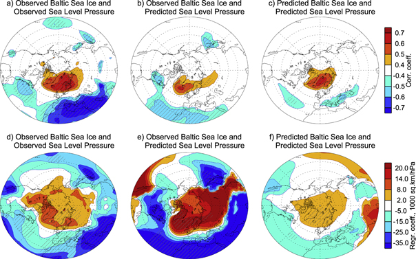
Figure 1. (Top) correlation and (bottom) regression coefficients between Baltic Sea MIE and DJF SLP for the period 1993–2012: (a), (d) observed MIE and observed SLP, (b), (e) observed MIE and GloSea5 predicted ensemble mean SLP; (c), (e) GloSea5 predicted MIE and SLP calculated across all individual members. Areas where absolute values of the correlation coefficient exceeds 0.44, which is statistically significant for 20 independent data pairs at p = 0.05, are hatched. Note irregular scale for the regression coefficients which is used to account for large variability of the polar SLP compared to the mid-latitude SLP.
Download figure:
Standard image High-resolution imageThe association between NAO and MIE suggests that skilful prediction of winter mean NAO may be sufficient to drive skilful MIE forecasts; indeed it may even be necessary. To confirm this we show in figure 1(b) correlation coefficients between observed MIE and ensemble mean DJF SLP predicted by GloSea5. Correlation coefficients in figure 1(b) are typically lower in magnitude than those in figure 1(a), and the centres of maximum correlations are located above the Atlantic Ocean, to the west of the observed ones. Also, the variability of the ensemble mean SLP is much lower than that in observations, which is reflected in a much larger regression coefficients between GloSea5 ensemble mean SLP and observed MIE compared to between observations SLP and MIE (figures 1(d) and (e)). The location of maximum correlations in figure 1(b) close to NAO centres of action (see e.g. Hurrell 1995) strongly suggests that the predictability of MIE in GloSea5 is mainly associated with model's ability to predict NAO, which justifies our approach to derive MIE predictive skill from NAO. We find a linear correlation coefficient between predicted NAOi and observed MIE of −0.51, with 95% confidence intervals 0.16–0.75, statistically significant at p = 0.01 according to a one-tailed t test, given that we know the expected sign of the correlation from observations. Defining NAOi as a SLP difference between Azores and Iceland, results in a similar correlation coefficient of −0.52, which indicates that the result is not sensitive to the definition of NAO.
To facilitate evaluation of MIE forecast skill we translate NAOi to MIE via regression. The MIE distribution is positively skewed as a result of negative skewness of winter temperatures, the absence of negative sea ice values and accelerated ice growth above the critical value of 180 000 km2 (Tinz 1996). Following previous authors, we seek an exponential relationship between NAOi and MIE, which accounts for stronger/weaker sensitivity of MIE to negative/positive NAOi values. Here, MIE = a × e−b×NAOi, where a and b are the regression coefficients to be found by a least square fit. Reliable estimation of the regression coefficients requires timeseries of sufficient length; therefore we fit this model to the observed MIE and NAOi values for the period 1950–1992, i.e. avoiding inclusion of the verification data to the regression model. Figure 2 shows that the resulting model provides a good fit to the observations for the whole period of observations from 1950 to 2012. Note that, because of the exponential relationship between NAOi and MIE, one could expect that periods of neutral to positive NAOi, when the sensitivity of MIE to NAOi is low should show reduced sea ice predictability compared to periods of negative to neutral NAOi when the sensitivity of MIE to NAOi is high. On the other hand, the spread of MIE around the exponential fit is larger for negative NAOi values, which reduces MIE predictability during negative NAOi conditions.
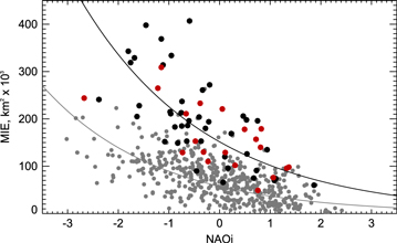
Figure 2. Scatterplot of MIE against NAOi in observations for the period 1950–1992 (black circles) and 1993–2012 (red circles) and GloSea5 ensemble members for the period 1993–2012 (grey circles). Solid lines are the regression model fits for observations (MIE = 152 × 103 × e−0.40×NAOi) and GloSea5 (MIE = 58 × 103 × e−0.44×NAOi).
Download figure:
Standard image High-resolution imageThe timeseries of MIE calculated based on GloSea5 NAOi is shown in figure 3 as well as observed MIE. The two timeseries correlate at 0.55 (95% confidence intervals are 0.21–0.77, significant at p = 0.012), i.e. the correlation between MIE and the exponent of NAOi is slightly higher than that between MIE and NAOi. This forecast explains about 30% of the observed MIE variance and we note that, to the best of our knowledge, this is the first documented skilful prediction of winter Baltic Sea ice conditions. The value of the forecasts can be further assessed by testing how skilful they are in predicting mild and severe ice conditions. Vainio (2011) analysed the 50-year period of MIE observations (1961–2010) and defined winters with MIE less than 115 000 km2 as mild ice winters, while those with MIE more than 230 000 km2 as severe ice winters. For the period 1961–2010 these thresholds approximately correspond to the 1st and 3rd quartiles of the MIE distribution. GloSea5 predictions of mild and severe ice winters are summarized in a contingency table (table 1) and illustrated in figure 3. For the results presented in table 1, the hit rates (defined as the proportion of occurrences that were correctly forecast) are 0.67 and 0.50, and the false alarm rates (defined as the proportion of non-occurrences that were incorrectly forecast) are 0.07 and 0.13 for the mild and severe ice winters, respectively. We note that for winters when observed mild (1992/93 and 2008/09) and severe (1995/96 and 2002/03) ice conditions were not predicted, the model predicted normal ice conditions, and not the conditions opposite to those observed, which would have more negative impact on the end users.
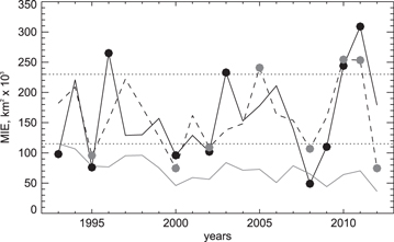
Figure 3. Timeseries of observed (solid black line) and GloSea5 simulated (grey line) Baltic Sea MIE. Dashed line shows MIE calculated from GloSea5 NAOi. Dotted lines indicate conventionally defined thresholds for mild and severe ice winters. Years with observed mild and severe ice conditions are indicated by black circles, and those predicted by GloSea5 are indicated by grey circles.
Download figure:
Standard image High-resolution imageTable 1. Contingency tables for Baltic Sea MIE forecasts (1993–2012). The numbers indicate the distribution of forecasts and observations obtained using conventional definition of mild and severe winters based on the observations from the period 1961–2010. The numbers in parentheses indicate the distribution obtained when mild and severe winters are defined in cross-validation mode using the data from the period 1993–2012 (see the text).
| Observed | ||||
|---|---|---|---|---|
| Forecast | Mild | Near normal | Severe | Forecast distribution |
| Mild | 4 (4) | 1 (1) | 0 (0) | 5 (5) |
| Near normal | 2 (2) | 7 (5) | 2 (3) | 11 (10) |
| Severe | 0 (0) | 2 (2) | 2 (3) | 4 (5) |
| Observed distribution | 6 (6) | 10 (8) | 4 (6) | 20 |
To test the sensitivity of the result to the definition of mild and severe winters we recalculate the thresholds using only the period 1993–2012 for which the forecasts are available. Specifically, we calculate the thresholds in a cross-validation mode leaving each winter in turn out and defining mild and severe ice winters as 5 winters with smallest and largest MIE among the remaining 19 winters, which approximately corresponds to the 1st and 3rd quartiles. The result, also presented in table 1, show only modest changes and essentially the same results for the hit rates and the false alarm rates, except that the false alarm rate for the severe winters increases to 0.14. Also, no one forecast of mild or severe ice winter is verified as an opposite category winter.
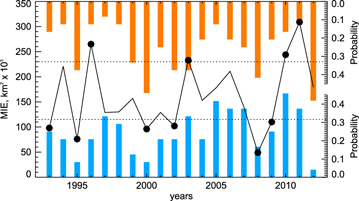
We further assess the quality of probabilistic sea ice forecasts using the spread among the GloSea5 ensemble members. Following the previous approach, we define mild and severe ice conditions as corresponding to the 1st and 3rd quartiles across GloSea5 ensemble members in a cross-validation mode and then calculate the fraction of ensemble members that predict mild and severe ice conditions for the left out winter. The forecast probabilities for mild and severe ice winters are shown in figure 4. The forecast probability of severe ice for the winters when severe ice condition were observed is, on average, 0.34, larger than its climatologically expected probability of 0.25. The corresponding number for the mild winters is also 0.34. At the same time the average forecast probability of mild (severe) winters when severe (mild) ice conditions was observed is 0.20 (0.17) only. The area under the relative operative characteristics (ROC) curve is a frequently used skill score of probabilistic forecasts in operational practices (Wilks 2006, Peng et al 2013). The ROC area for the forecasts of mild and severe ice conditions is 0.79 and 0.76, respectively. In both cases it is larger than 0.5, which indicate a positive skill. These results corroborate our conclusion about skilfulness of the GloSea5 sea ice forecasts.
Figure 4. Timeseries of observed (solid black line) Baltic Sea MIE. Dotted lines indicate conventionally defined thresholds for mild and severe ice winters. Years with observed mild and severe ice conditions are indicated by black circles. Bar chart indicates probabilities of mild (orange) and severe (blue) ice conditions calculated from GloSea5 ensemble members (note the reversed axis for the mild winter probabilities).
Download figure:
Standard image High-resolution image
We also tried to directly utilize the GloSea5 predicted Baltic Sea ice. MIE calculated from the GloSea5 simulated ice cover is biased low as can be seen in figure 3. Moreover the correlation with the observed MIE is only 0.04. Figure 3 also reveals a significant negative trend in simulated MIE, the reasons of which are not known yet. There is no significant trend over the same period in observations, but note the observations also have a much larger variance. Moreover, Luomaranta et al (2014) did not find a statistically significant trend in MIE over the longer period 1901–2013. Removing the simulated trend from the GloSea5 MIE slightly improves the correlation with observations to 0.29 but the skill remains low.
To get some insight into why GloSea5 explicitly simulated Baltic Sea ice has low predictive skill we now discuss the correlation between simulated SLP and MIE plotted in figure 1(c). Although the relation is quantitatively similar to the observed one, the magnitude of the correlation is substantially weaker. The weaker correlation can, at least partly, be attributed to the low bias in simulated MIE. As can be seen in figure 2, near ice-free conditions are simulated by GloSea5 over a broad range of NAOi values, so that Baltic Sea ice in the model becomes less sensitive to increases in heat advection associated with increases in NAOi. The low value and low variance of the sea ice in the forecast model is due to a warm SST bias over the Baltic Sea by about 0.5–1.0 °C in regions of ice deficit. The exact causes of this bias is under investigation, however, the global ocean model with the ORCA0.25 grid was never optimized for performance over shallow seas, and although surface waters will be suitably initialized by satellite SST and the overlying atmospheric temperature, subsurface layers will not be as suitably constrained. Since sea ice formation is inherently a threshold process, the warm bias decreases both the mean sea ice coverage and it's variability. Moreover, Scaife et al (2014) noticed that in GloSea5 the predicted NAO is a better predictor of Northern European winter temperatures than the predicted temperatures themselves because of imperfect NAO teleconnections, such as NAO impacts on Northern European temperatures, in the model, perhaps related to the small amplitude of the ensemble mean signal (cf Eade et al 2014).
Finally, we assess the potential predictability of Baltic Sea ice within GloSea5, which is defined as the mean correlation coefficient between ensemble mean and each individual ensemble member (e.g. Kumar et al 2014). The potential predictability of MIE calculated from NAOi is 0.16, much lower than the actual predictability of 0.55. This is expected result given that previously Scaife et al (2014) and Eade et al (2014) found low potential predictability in GloSea5 NAOi predictions. Note that the potential predictability estimated from the dispersion of ensemble members cannot be interpreted as the upper limit of achievable predictability (Kumar et al 2014). In fact, low potential predictability compared to actual predictability indicates anomalously low signal-to-noise ratio in the model forecasts and implies that the forecast skill of both the NAO and Baltic Sea Ice could be further increased by increasing the number of ensemble members (Scaife et al 2014).
Discussion and conclusions
Wintertime navigation in the Baltic Sea is continually growing (Vihma and Haapala 2009) and so does the need for skilful sea ice forecasts. Currently, operational services provide forecasts of sea ice conditions for a few days only (Vihma and Haapala 2009). Here we report the first skilful predictions of annual maximum Baltic Sea ice extent (MIE) using output from the GloSea5 forecast system. For the 20-year period (1993–2012) the forecast skill measured by correlation coefficient is 0.55, the hit rate for forecasts of mild (severe) ice winters is 0.67 (0.50) and the corresponding false alarm rate is only 0.07 (0.13). Such a skill level may be useful for practical applications.
This skill is derived from the predictability of the North Atlantic Oscillation because, as we show, the simulated Baltic Sea ice extent itself has little predictive skill. The lack of skill can be partly explained by the low bias in the mean simulated MIE, which weakens the sensitivity of the sea ice to variations in atmospheric circulation of the model. This result also implies that the predictability of MIE from NAOi would reduce in a warmer climate as a result of climate change.
As discussed in Scaife et al (2014) the sources of NAO predictability in GloSea5 include El Niño/Southern Oscillation (Toniazzo and Scaife 2006), Kara sea ice autumn anomalies (Yang and Christensen 2012) and Atlantic ocean heat content (Rodwell and Folland 2002). The NAO predictive skill found here and in the previous studies (Scaife et al 2014) is consistent with earlier investigations of statistical properties of the observed NAO timeseries and European temperatures (Stephenson et al 2000, Keeley et al 2009, Folland et al 2012). At the same time it remains unclear to what degree the European climate variability not related to NAO is predictable at seasonal scale. It cannot be excluded that non-NAO variability of the Northern European climate, in particular of Baltic Sea ice, represent climatic noise, and so contaminate the predictable signal associated with NAO. One interesting possibility for further development is to investigate whether the predictive skill of Baltic Sea ice can be derived from the Pacific Decadal Oscillation (PDO), which has recently been found to influence Baltic Sea ice variability (Vihma et al 2014). In any case, our current results suggest that the NAO represents an important source of predictability for the wintertime Baltic Sea ice conditions.
Acknowledgments
We thank two anonymous reviewers for their valuable comments. We acknowledge NCEP/NCAR for providing their reanalysis data and ECMWF for providing Era-Interim reanalysis data. The contribution of AYK is funded by FMI's tenure track program. AAS and KAP were supported by the Joint DECC/Defra Met Office Hadley Centre Climate Programme (GA01101), the UK Public Weather Service research programme, and the European Union's Framework 7 Programme (FP7/2007-2013) under the SPECS project (Grant Agreement 308378).