

Abstract
Mapping anthropogenic forest disturbances has largely been focused on distinct delineations of events of deforestation using optical satellite images. In the tropics, frequent cloud cover and the challenge of quantifying forest degradation remain problematic. In this study, we detect processes of deforestation, forest degradation and successional dynamics, using long-wavelength radar (L-band from ALOS PALSAR) backscatter. We present a detection algorithm that allows for repeated disturbances on the same land, and identifies areas with slow- and fast-recovering changes in backscatter in close spatial and temporal proximity. In the study area in Madre de Dios, Peru, 2.3% of land was found to be disturbed over three years, with a false positive rate of 0.3% of area. A low, but significant, detection rate of degradation from sparse and small-scale selective logging was achieved. Disturbances were most common along the tri-national Interoceanic Highway, as well as in mining areas and areas under no land use allocation. A continuous spatial gradient of disturbance was observed, highlighting artefacts arising from imposing discrete boundaries on deforestation events. The magnitude of initial radar backscatter, and backscatter decrease, suggested that large-scale deforestation was likely in areas with initially low biomass, either naturally or since already under anthropogenic use. Further, backscatter increases following disturbance suggested that radar can be used to characterize successional disturbance dynamics, such as biomass accumulation in lands post-abandonment. The presented radar-based detection algorithm is spatially and temporally scalable, and can support monitoring degradation and deforestation in tropical rainforests with the use of products from ALOS-2 and the future SAOCOM and BIOMASS missions.
Export citation and abstract BibTeX RIS

Content from this work may be used under the terms of the Creative Commons Attribution 3.0 licence. Any further distribution of this work must maintain attribution to the author(s) and the title of the work, journal citation and DOI.
1. Introduction
There is wide international agreement on the critical role of forests in mitigating climate change. Reducing emissions from deforestation and forest degradation, with conservation, sustainable management and enhancement of forest carbon stocks in developing countries (REDD+), has been under intense negotiation since 2007 (UNFCCC 2007, 2011). Alongside this process, monitoring forests using satellites is gaining pace as studies progress in assessing carbon stocks and forest clearance across the globe (Houghton and Goetz 2008, Baccini et al 2012, Hansen et al 2013).
Of particular interest to forest monitoring is detecting degradation, i.e. the anthropogenic reduction of forest cover or woody biomass in areas that still remain defined as 'forests' of more than 10–30% tree cover (FAO 2002). In contrast to deforestation, which can be identified based on classifications of forest into changed/unchanged, degraded forests can be in any state along a 'bare-ground' to 'intact-forest' continuum based on numerous definitions (Schoene et al 2007, Sasaki and Putz 2009, Guariguata et al 2009). Studies that quantify carbon emissions or the extent of degradation indicate that it is widespread across the tropics and affecting land area similar to, or of larger portion, than deforestation (Asner et al 2010, Margono et al 2012, Zhuravleva et al 2013, Ryan et al 2012, 2014, Pearson et al 2014). Since degradation has been shown to precede deforestation (Ahrends et al 2010, Asner et al 2006), quantifying the former may assist the prevention of the latter. While distinct conceptualizations of the two spatially and temporally correlated processes may challenge efforts towards characterizing anthropogenic forest disturbances, standard conceptualizations based on binary land classification (Lu et al 2005) also broadly risk oversimplifying the process of degradation. The challenge arises since degraded areas are often dynamic frontiers in transition, and may recover or be repeatedly disturbed before being deforested.
The southwestern Peruvian Amazon, including the region of Madre de Dios, is important in this context. It is recognized as a tropical 'Capital of Biodiversity' (Peruvian law No. 26311) and a conservation priority (Myers et al 2000) since it has been threatened by deforestation and degradation following the paving of the tri-national interoceanic highway (IOH) since 2006 (Southworth et al 2011, Kirkby et al 2011). High-accuracy automated methods that utilize multi-temporal Landsat satellite imagery to map deforestation (Asner et al 2009, Hansen et al 2013, Potapov et al 2014) are widely used in Peru. However, these methods are often restricted to cloud-free conditions since they rely on an optical sensor. Over three-quarters of intact tropical forests have over 70% cloud cover on average (calculated for years 2010–2014 (NEO 2015)), particularly in Papua New Guinea, Borneo, Sumatra, Gabon and the North-Western Amazon. Hence, obtaining regular cloud-free imagery from satellites with low repeat coverage per year is rare in many areas (Asner 2001, Chambers et al 2007). Optical-derived vegetation indices typically used in mapping biomass or leaf area have also been shown to saturate in dense forests (Asner et al 2004, Song 2013), challenging the detection of subtle changes in vegetation structure. Spaceborne radar imagery operating at microwave frequencies instead offers the advantage of being unaffected by cloud and atmospheric effects, and allowing night-time acquisition. Long-wavelength radar signals can penetrate canopies (Rignot et al 1995, Wang et al 1998, Woodhouse 2006a) and have been related to forest structure and woody biomass (Woodhouse et al 2012) up to a saturation limit (higher for longer wavelengths), which allow them to be used in support for land use monitoring (Ryan et al 2014). Additionally, radar has been used to detect changes in biomass resulting specifically from degradation (Mitchard et al 2011, Ryan et al 2012, Mitchard et al 2013, Ryan et al 2014). Despite its numerous advantages, the cost and limited availability of long-wavelength radar imagery, and the sensitivity of the signal to surface topography and moisture, has restricted establishing it as a method to study forest disturbances.
Our research demonstrates a method to detect forest cover change dynamics, including degradation, deforestation and succession, using annual radar images from 2007 to 2010. The analysis includes secondary and degraded forests, since this broad definition accommodates for the detection of repeated use of land. We distinguish intact forest as consisting of native tree species and ecological processes that are not visibly affected by humans (Potapov et al 2008). Further, so as to not arbitrarily delineate deforestation and degradation, we define forest disturbance as including both the effects of clear-cutting from deforestation and diffuse forest cover loss from degradation. Forest disturbances are studied by mapping and analysing differences in radar backscatter (L-band at 24 cm wavelength), i.e. the proportion of outgoing radar power that bounces back to the satellite from the ground (Woodhouse 2006a), between years. Decreases in backscatter have been previously reported to correspond to canopy cover reduction (Thiel et al 2006, Ryan et al 2012), while increases are dependent on management practices and are expected with canopy cover recovery (e.g. after selective logging (Asner et al 2006)). Here, we interpret a drop in backscatter as forest disturbance, and a recovery of backscatter values in the years thereafter as successional forest dynamics (sensu Christensen 2014). The output disturbance maps allow us to ask the following question: can the analysis of radar backscatter intensity provide information on (a) the spatial distribution and (b) the dynamics of forest disturbances in tropical rainforests?
2. Land cover and use in the study area
Our study covers parts of Tahuamanu and Tambopata provinces of Madre de Dios (figure 1(a)). Natural ecosystems of tropical forests cover 80% of the area, including lowland rainforests and extensive thickets of arborescent bamboo on alluvial terraces and floodplains. Other natural ecosystems cover less than 5% of the region, including palm swamps (3%) and rivers (2%). Annual precipitation exceeds 1500 mm, received mostly from November to March (figure S1 in the supplementary data, available at stacks.iop.org/erl/10/034014/mmedia).
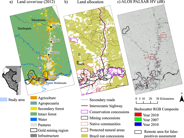
Figure 1. (a) Land cover/land use map of the study area, produced by visual interpretation of Resouresat imagery (25 × 25 m) from 2012 and ground-data collected in 2013 (IIAP 2013, BAM 2013). The mining region was identified using WorldView-2 imagery from July 2011. 'Agropecuaria' are areas of a mix of secondary forests, pastures and agriculture. (b) Designated land use concessions in the study area. (c) ALOS PALSAR backscatter ( ) for years 2010 and 2007 as an red, green, blue colour composite. Area A is illustrated in figure 4, and B and C in figure S8.
Download figure:
Standard image High-resolution imageDuring the study period, the region was deforested at an estimated rate of 0.35% yr−1 (Hansen et al 2013) due to (i) clearance for subsistence agriculture farms of sizes between ∼1 and 10 ha (ii) clearance for pastures of sizes between ∼1 and 40 ha, commonly abandoned since cattle-ownership was low; and (iii) illegal clandestine gold-mining (figure S2). Conservation priorities are well recognized (Kirkby et al 2010) and forest concession systems (Brazil nut, conservation, ecotourism and indigenous lands) have had inhibitory effects on deforestation in the region (Nunes et al 2012, Vuohelainen et al 2012). However, overlapping and conflicting land use allocations have increased land pressure (Scullion et al 2014) (figure 1(b)).
The sustainability of selective timber harvesting in Brazil nut concessions has drawn attention since a 5 m3 ha−1 cap on extraction was lifted in 2007 (Giudice et al 2012). Extraction is common in drier months, but personal observations (Woo 2012) recorded timber-trucks exiting forests throughout the year. Although extraction rates were highest in the 2007–2008 period of this study, exceeding those in allocated timber concessions of Madre de Dios, they remained below 3.7 m3 ha−1 on average (Cossío-Solano et al 2011).
3. Material and methods
3.1. Radar scenes
Surface moisture can vary backscatter and decrease its contrast over forests and bare-ground. To minimize the problem, two dry-season scenes were acquired from the phased array L-band Synthetic Aperture Radar sensor aboard the Advanced Land Observing Satellite (ALOS PALSAR) in July–August for each year from 2007 to 2010 (scene IDs provided in table S1). Since terrain can significantly impact image projection and backscatter, scenes were terrain-corrected and radiometrically calibrated using the 90 m resolution Shuttle Radar Topography Mission dataset (Jarvis et al 2008). They were then converted to backscatter (co-polarized  and cross-polarized
  ) using coefficients of Shimada et al (2009) and mapped at 15 m resolution in UTM projection (schematic processing chain is shown in figure 2(a)).

Figure 2. (a) Pre-processing of ALOS PALSAR images. RFDI is the Radar Forest Degradation Index (Mitchard et al 2012). (b) Distribution of uncalibrated and (c) calibrated annual  values (in power domain) to the base year 2007. SD refers to standard deviation.
Download figure:
Standard image High-resolution imageSpeckle, which is inherent in radar images (Woodhouse 2006a), may be problematic for accurate disturbance detection. Our images were moderately despeckled using the Enhanced Lee Filter (Lopes et al 1990) with a 3 × 3 pixel window to retain textural information. Image pixels were then averaged to 30 m resolution as a compromise to reduce speckle, but allow the detection of small-area disturbances and comparability to Landsat-based deforestation datasets (e.g. Asner et al 2010, Hansen et al 2013).
To reduce any remaining variability in backscatter unrelated to anthropogenic disturbances, images were calibrated to the base year (2007) by adjusting pixel values by the difference in average backscatter over a 510 × 510 m window (figures 2(b)–(c)). This procedure was chosen since it showed reasonable adjustment over known forest/non-forest areas (collected field data described in section 3.2.2), and corrected for variations over different land cover types locally. The chosen window size was much larger than most known disturbances in the region, and they were hence unlikely to be lost by the calibration. To ensure that large-area disturbances were not lost, backscatter was not adjusted if averages differed by more than a cut-off threshold; here, half the standard deviation of 2007 backscatter, chosen empirically based on field knowledge of large-area disturbances. The procedure showed no significant impact on the area-dependent analysis presented in section 4.4.
3.2. Mapping forest disturbances
3.2.1. Detection algorithm
A preliminary investigation of our study region revealed frequently disturbed areas with a continuum of surrounding disturbed land. To maximize the detection of these areas, we exploited the advantage of multi-temporal and spatially continuous radar images. A time-series allows the same pixel to be observed multiple times, and hence allows more confidence in determining its status (disturbed/undisturbed), as compared to only two observations. To minimize detecting backscatter variations unrelated to anthropogenic disturbances, we used a local moving-window filtering procedure that assumes that disturbances are more likely to be real if they neighbour other disturbances. The designed algorithm hence (i) uses multi-temporal data as intermediate information to verify disturbance locations, but does not temporally categorize change pixels initially, and (ii) identifies areas with slow-recovering and fast-recovering backscatter change (i.e. areas where backscatter remained consistently changed compared to year 2007 for a period of two years or more, and for a period of one year, respectively) in close proximity, but does not spatially categorize these into deforested/degraded.
Areas known to have <30% forest cover in year 2000 (Hansen et al 2013),  −14.0 dB or Radar Forest Degradation Index >0.5 (figure 2(a)) (Mitchard et al 2012) in 2007 were discarded, removing bare-ground, infrastructure, water and some inundated swamps (4.7% of study area) from the analysis. Sucessional forest dynamics are not studied for these areas. Backscatter, particularly
  , was found to be related to biomass for the remaining areas (figure S3) and observed to decrease upon disturbance. Since forests tend to depolarize the radar signal (Woodhouse 2006a), giving high
  values that reduce upon forest cover loss, our methodology uses the annual loss in
  for disturbance detection.
To identify a disturbed pixel, the algorithm uses a set of thresholds (T1 to T5, table 1), explained in figure 3 and exemplified in figure 4. Five backscatter change maps ( –
– ,
,  –
– ,
,  –
– ,
,  –
– and
and  –
– ) were produced and disturbance captured in two stages. First, slow-recovering changes are selected by eliminating pixels with change values that do not meet threshold T1 and are not seen consistently over two years or more (box A, output 1), and are spatially isolated from pixels detected in all years' slow-recovering change maps (output 2). Second, fast-recovering changes are selected by eliminating pixels with change values that do not meet threshold T1 (box B, output 3), and eliminating pixels that are spatially isolated from all years' fast-recovering or slow-recovering change maps (output 4). Locations of disturbances are then assigned to time periods to obtain annual disturbance maps (box C, output 5).
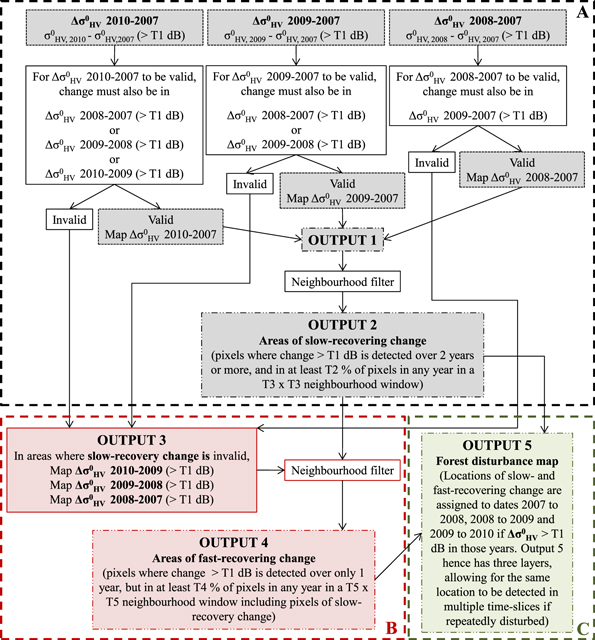
Figure 3. Forest disturbance detection algorithm using ALOS PALSAR backscatter ( in dB). Slow-recovering changes are detected first (box A) and fast-recovering changes located in distant areas, as well as in close spatial and temporal proximity to slow-recovery changes, are then detected (box B). T1, T2, T3, T4 and T5 are thresholds set based on training data through an empirical manual process. An illustrative example of the algorithm is shown in figure 4.
Download figure:
Standard image High-resolution image
Figure 4. Illustrative example of disturbance detected in area A, figure 1(c), with pixels values of  or
or  in dB shown as red, green, blue (RGB) colour composites. Black areas show no disturbance, and non-forest areas before July 2007are shown in white. Outputs 1–5 are described in the schematic disturbance detection algorithm in figure 3.
Download figure:
Standard image High-resolution imageTable 1. Thresholds selected for forest disturbance detection in the study area for the algorithm presented in figure 3. Thresholds were chosen empirically through a manual process, aimed at maximizing detecting known disturbances and minimizing false detections based on prior knowledge of the study area.
| Threshold | Chosen value |
|---|---|
| T1 | −1.5 dB |
| T2 | 56% |
| T3 | 2 pixels |
| T4 | 67.5% |
| T5 | 3 pixels |
3.2.2. Training and validating detections
Thresholds for removing non-forest areas, and T1–T5 (table 1), were chosen empirically through a manual iterative process, aimed to minimize false detections and maximize detecting known disturbances. The latter were obtained from a visual inspection of (i) GeoEye-1 images from July 2011 and Google Earth, (ii) 107 ground-locations of forest and non-forest areas obtained over 2011–2013 (figure S4), and (iii) the yearly Asner et al (2010) and Hansen et al (2013) forest loss maps (available at MINAM (2014) and UMD (2013)).
Multiple products (figure S4) were used to validate the disturbance maps:
- (1)Fifty-six new agriculture and pastoral farms of 0.25–90 ha were visually identified using Landsat (July 2007) and Resourcesat (August 2010) imagery. Farm locations were verified using Google Earth and their edges manually digitized to polygons using a WorldView-2 image (2 m resolution) from July 2011. A hit rate and miss rate was derived, defined as the number of pixels in the polygons that were caught and lost on the disturbance maps respectively. A 3 × 3 window majority filter was used to fill gaps within detected areas before this analysis.
- (2)False positives were quantified by analysing a 5219 ha area of the region that had no recorded logging and no detections on previous forest loss datasets (Asner et al 2010, Hansen et al 2013) (figure 1(c)). Using this definition of false positives is a conservative estimate, as it relies on the absence of anthropogenic disturbance and may include unquantified natural disturbances.
- (3)Records of volumes of roundwood harvest in Brazil nut concessions were obtained from 2008 to 2010 (ATFFS 2011) and related to the area detected.
- (4)Ground-GPS locations of 24 requested harvest areas of 26–690 ha in 2010 were compared against detections.
- (5)Thirty-four GPS locations of 1–3-year-old felling gaps were acquired during June–August 2011 and compared against detections. Gap sizes ranged 120–290 m2, leaving canopy openness of ∼20% (Moll-Rocek et al 2014).
A Monte Carlo procedure was used to estimate the probability of detecting the 24 logging areas and 34 felling-gaps by chance, by simulating random disturbances in the extent of the Brazil nut concessions where these observations were made in 1000 iterations (mathematical description in supplementary information). A sensitivity analysis of the hit rate and false positive rate to the thresholds T1–T5 was then conducted by varying them independently.
3.2.3. Estimating false positives due to speckle
To test the contribution of speckle to false detections, we simulated annual datasets of homogeneous forest with random noise over 106 pixels. Statistical parameters of the distribution were set by analysing the same area as for false positives, i.e. mean equal to the average annual backscatter and variance to half the average variance of backscatter differences between years, to mimic the additive noise contribution of speckle (mathematical description in supplementary information). The disturbance detection algorithm was then run for 100 iterations to quantify percent of pixels detected by chance.
4. Results
4.1. Forest disturbances
Significant differences in the distribution of backscatter for disturbed and undisturbed, and slow- and fast-recovering, areas were recorded in the study region (figures 5(a)–(b)). Over the three year period, 2.3% (17 722 ha) of the study area was disturbed (rate of 0.78% yr−1), with 1.3% under slow-recovery and 1.0% under fast-recovery. Of the disturbed land, 2,555 ha was found to be repeatedly disturbed during the three years, and there was decline in total disturbed area with each year (table 2). Disturbances were observed mostly along the IOH and secondary roads, although fast-recovering disturbances were more widespread (figure 5(c)).
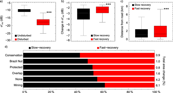
Figure 5. (a) Distribution of radar backscatter in disturbed and undisturbed areas. (b) Distribution of change in backscatter for areas of fast-recovering and slow-recovering backscatter following disturbance. (c) Spatial distance of disturbances from secondary and primary roads in study area. (d) Fraction of slow- and fast-recovering changes in selected land concessions (figure 1(b)) in the 2007–2010 period. 'None' refers to areas with no designation, primarily lands already in use for agricultural purposes. 'Overlap' refers to all designations that overlap mining concessions. Significance of difference is provided as p-value *** <0.001.
Download figure:
Standard image High-resolution imageTable 2. Extent of forest disturbances detected using radar in the study region.
| Area of disturbance (hectares) | (percent of study area) | |||
|---|---|---|---|---|
| Period | Slow-recovery | Fast-recovery | Total | % |
| Jul 2007–Aug 2008 | 3,743 | 4,148 | 7,891 | 1.05 |
| Aug 2008–Jul 2009 | 5,101 | 2,231 | 7,331 | 0.97 |
| Jul 2009–Jul 2010 | 3,032 | 2,022 | 5,055 | 0.67 |
The proportion of change type (fast- and slow-recovering) differed over areas with different authorized land uses (figure 5(d)). Protected areas, conservation and Brazil nut concessions had the lowest percent of forest disturbance, and a higher fraction of fast-recovering changes, in comparison to mining concessions and areas under no allocated land use (e.g. lands in long-term use for mainly agricultural and pastoral farming).
4.2. Detection validation and algorithm sensitivity
Validation of the detection algorithm is reported using the sources introduced in section 3.2.2:
- (1)Disturbances were detected in 1721 of 2740 pixels on the delineated agricultural and pastoral farms, a hit rate of 63% and miss rate of 37%, over the three years.
- (2)Over the remote forest area, the difference in backscatter was 0.015 ± 1.477 dB (mean ±standard deviation) between 2007 and 2010 (figure S5). A false positive rate of 0.3% of area was detected (consistently 0.1% yr−1). Of these, slow-recovery false positives were 0.04% of area, suggesting that there is more uncertainty associated with fast-recovering disturbances. Sensitivity of detections to simulated speckle (section 3.2.3) showed that only a small proportion of pixels, 0.04% yr−1, are detected by chance. This suggests that at least some false positives in the remote area are genuine disturbances.
- (3)Of the 250 Brazil nut concessions that reported logging, disturbances were detected in 212 concessions. For these, regression analysis between extracted volumes normalized by concessions' area and percentage of detected disturbed area showed a very weak but significant relation, particularly for the last year of data (r2 = 0.15, p < 0.001) (figure S6). Disturbances are not expected to result from logging activities alone and log volumes do not necessarily have a high correlation with area logged. However, the result suggests that the area of detections picked up by radar are realistic to a significant extent.
- (4)Of the 24 GPS-marked areas where logging permission was requested, disturbances were observed within 12, and in 15 when allowing for a 90 m buffer (threshold T5). The probability of these 15 being observed by chance is 0.04 or 4% (i.e. in 40 of 1000 iterations).
- (5)Of the 34 felling gaps however, only 6 were detected within 60–90 m buffer with a probability of chance observation of 0.01 or 1% (i.e in 10 of 1000 iterations). The low detection rate is expected, since logging is sparse in the region and felling-gaps are smaller than the radar image resolution (Moll-Rocek et al 2014).
The sensitivity analysis to thresholds T1–T5 showed that the algorithm was most sensitive to T2 and T4, i.e. the fraction of pixels that must be disturbed within the neighbourhood of a pixel for it to be selected as disturbed, followed by T3 and T5, i.e. the neighbourhood size. A 0% false positive rate was achievable, although at the expense of reducing the hit rate to between 50 and 52% (figure S7).
4.3. Spatial pattern of disturbances
To analyse the spatial patterns of detections, disturbances were visualized as forest disturbance 'events' (FDE) by grouping and converting neighbouring disturbed pixels to polygons. These polygons indicated that 85% of slow-recovery events were detected with fast-recovery events along edges, visibly related to the same land use. Fast-recovery events were more frequent (2.6 times) than and more isolated from slow-recovery events (70% neighboured slow-recovery events). Both types of disturbances were also common at the frontiers of already-cleared land (figures 4 and S8). It was noted that spatially delineating disturbed areas with abrupt boundaries risks ignoring surrounding lands in transitional disturbance. Hence, we fused neighbouring fast- and slow-recovery events as belonging to the same FDE, merging neighbouring deforestation and degradation and giving a continuous spatial gradient of disturbance.
4.4. Disturbances by land use
To understand successional forest dynamics, we analysed fused FDEs occurring in the 2007–2008 period that fall into different land cover/use categories, delineated using an independent dataset in 2012 (figure 1(a)) (IIAP 2013, BAM 2013). Analysis of variance (ANOVA) tests revealed that events resulting in pastures, typically clearing full forest cover, were characterized with significantly lower backscatter prior to disturbance as compared to (unclassified) events in intact forests (difference of 1.1 dB, p < 0.001) and gold-mining (difference of 0.8 dB, p < 0.001) (figure 6). Such a result is expected, as pastures are concentrated along areas already under human-use (figure 1(a)) and gold-mining involves clearing relatively intact forests. Backscatter remains low in successive years following FDE for gold-mining as compared to increases observed for events in intact and secondary forests (difference of 1.5 and 1.2 dB respectively, p < 0.001), suggesting that the recovery of forest cover or biomass in gold-mining areas is significantly slower (test statistics described in tables S2–S4).

Figure 6. Distribution of backscatter in forest disturbance events detected in the 2007–2008 period, classified by land use/cover (figure 1(a)). Outliers in data are not shown. Summary of analysis of variance (ANOVA) test statistics of the differences between categorized data means are provided in tables S2–S4.
Download figure:
Standard image High-resolution imageInitial and recovered backscatter values were also related to the size of land cleared for each land use (examples in figure 7). Regression analysis revealed that (i) large-sized events for pastures and gold-mining begin with low backscatter in the year before clearance (slope = −0.51 and −0.47 respectively, p < 0.001), suggesting that the clearing of large areas is more common in lands with low biomass. Although a similar trend is visible in intact forests, the overall trend across events of different sizes is not significant (p > 0.5); (ii) large-sized events also have a large drop in backscatter during a FDE, particularly for gold mining (slope = −0.96, p < 0.001). The magnitude of change (ranging ∼3–5 dB) suggests that these large-areas are more likely to be fully cleared or with very low biomass immediately after disturbance. In contrast, small-sized events are more likely to be diffuse disturbances not involving full clearance; and (iii) large-sized events for pastures, and marginally for gold-mining (slope = 0.37, p = 0.02), recover backscatter faster in the years after FDE. Personal field observations (Woo 2012) recorded that parts of large pastures were commonly abandoned due to maintenance challenges. Small changes in biomass may cause large changes in backscatter when initial biomass values are low, as seen theoretically (Woodhouse 2006b, Brolly and Woodhouse 2012) and empirically (non-linear biomass-backscatter curve, figure S3). The result suggests that rapid cover and biomass accumulation post-disturbance are crucial successional dynamics in these lands.

Figure 7. Distribution (box plots) and means (black circles) of backscatter values for forest disturbance events of various sizes detected in the 2007–2008 period for three land use/cover types. Data is binned into intervals of area (hectares) in logarithmic scale for the visualization of trends. Regression parameters are for a linear least squares regression with area (in hectares) in logarithmic scale, since this ensures homogeneity of residual variance. Outliers in data are not shown.
Download figure:
Standard image High-resolution image5. Discussion
5.1. Detecting disturbances in tropical forests with radar
Our study presents a new algorithm to detect forest disturbances using radar, relying on a temporal trajectory of backscatter change and identifying areas with both slow-recovering (backscatter drop sustained for two or more years) and fast-recovering (backscatter drop sustained for one year) disturbances. In the rainforests of Madre de Dios, we estimated that 2.3% of the study area was disturbed between July 2007–2010 with a false-positive rate of 0.3% of area, and with disturbances most widespread during July 2007–August 2009. This peak is similar to that noted in previous studies (Asner et al 2010, Hansen et al 2013), and has been linked to the boom of international gold prices in 2008–2009 and increasing land use by migrants (Fraser 2009, Swenson et al 2011, Vuohelainen et al 2012, Asner et al 2013). Similar to previous studies, protected, conservation or sustainably managed areas were least disturbed, either due to the inhibitory effects of land concessions on deforestation or their remote location (Nunes et al 2012, Vuohelainen et al 2012).
Comparisons to optical-based deforestation datasets of Asner et al (2010) and Hansen et al (2013) however indicated that the total area of disturbance detected by radar, summing fast- and slow-recovering areas, is over twice their estimates (after removing pixels overlapping detections occurring before 2007 in both previous studies) (figure 8(a)). This is not necessarily a like-for-like comparison, as the studies demarcate annual forest loss and may exclude the observed extended gradient of disturbances surrounding affected areas (examples in figure S8) (although Asner et al (2010) includes 'disturbances', there are diffuse thinning from other land uses). We allowed for ±1 year buffer in the temporal classification of forest disturbance events and assessed the number of events that overlapped between studies by at least 25% of area. Most differences were for small-sized events, i.e. <30% of previous studies' events of 0.3 ha and 70% at 1.7 ha were detected in our map (figure 8 (b)). At ∼4 ha the Hansen et al (2013) study captured 50% and the Asner et al (2010) study captured 30% of our events (figures 8 (c)–(d)).

Figure 8. Comparison of radar-based forest disturbance detection to Asner et al (2010) andHansen et al (2013) deforestation maps. Detections in the present study that occurred prior to 2007 in the other datasets were removed, reducing the total changed area on our maps by 27, 18 and 16% in 2007–2008, 2008–2009 and 2009–2010 (compared to area presented in table 2). The Asner et al (2010) data includes both deforestation and diffuse forest thinning. (b) Shows the fraction of detections in the previous studies captured in the present study and the Asner et al (2010) diffuse thinning is referred to as 'disturbance', while (c) and (d) show fraction of the present study detections captured in previous studies, with an event area overlap of at least 25%. Data is binned into intervals of area (hectares) in logarithmic scale to visualize trends.
Download figure:
Standard image High-resolution image
The comparability of the performance of the datasets is limited, since we only assess end-products of optical-derived regional to global deforestation and our study targets mapping accurate provincial-level disturbances backed by detailed field-surveys instead. However, long-wavelength radar is expected to detect larger areas of disturbance, including degradation, mainly due to its sensitivity to changes within and below the forest canopy. Relations between disturbed area and timber-extract volumes and locations suggest that degradation is picked up to a significant extent in Madre de Dios. Some studies have relied on a combination of data, such as optical and airborne/satellite lidar (e.g. Asner et al 2010, Zhuravleva et al 2013), to specifically capture degradation. We hence urge the development of methods that integrate radar in such studies to aid frequent disturbance monitoring. However, constraints still remain on the availability, extent and costs of long-wavelength radar imagery, which may be overcome with products from ALOS-2 (JAXA 2014) and the future SAOCOM (CONAE 2014) and BIOMASS (LeToan et al 2011) missions.
5.2. Limitations of disturbance detection algorithm
Various scattering processes associated with land disturbances have shown to cause both decreases and increases in backscatter (Whittle et al 2012). In our study area, an examination of known disturbances showed that a loss in the cross-polarized signal,  , dominated over disturbed lands. This is expected, since processes that may increase backscatter and cause large changes in the co-polarized signal (e.g. creating and maintaining hard forest edges for ranches) were not common practices. Further, backscatter may have low sensitivity to low-magnitude biomass losses in areas with high biomass due to apparent signal saturation (typically 100 Mg ha−1 for L-band radar). However, significant detections including selective logging were picked up in such areas. This may be because large disturbances in vegetation structure that were relevant at the 30 m resolution (e.g. removal of a large tree), and to which backscatter is fundamentally related (Woodhouse et al 2012), accompanied these activities. Broadly, further research on backscatter–vegetation interactions and potential errors from saturation would greatly benefit the use of radar for disturbance detection over other study areas.
Limitations also lie in needing to set cut-off thresholds T1–T5 (table 1) in the algorithm. The algorithm performance was most sensitive to the spatial extent of disturbances. The thresholds inherently coarsen the output map 'resolution', losing very small-sized or slow biomass losses, and resulting in a miss rate of known disturbances of 37% and low detection rate of gaps from sparse selective logging. However, the algorithm is designed using a sequence of observations to ensure confidence in results. Inserting 'time-slices' of more frequent image acquisitions, such as those from the 14-day repeat cycle of ALOS-2, can allow for more flexibility in the use of thresholds. Nevertheless, environmental conditions such as soil moisture, changes in understory vegetation, sensor calibration drift and speckle are expected to contribute to noise and false positives, requiring local-calibration and ground-data to ensure accuracy.
5.3. Benefits for REDD+ and land monitoring
Since deforestation and forest degradation may not constitute simple land cover conversions between two time periods, the radar-based change detection algorithm improves the characterization of these processes by allowing for fluctuations and reversibility in conversion, and the detection of repeated disturbances. A significant proportion of fast-recovering disturbance events (70%) neighboured slow-recovering events. This result highlights both the continuous gradient of land cover change (Guariguata et al 2009) and the possibility of degradation preceding and accompanying deforestation. While a recent synthesis of national REDD+ readiness revealed that most countries' direct intervention plans focus on reducing forest degradation (Salvini et al 2014), methods to quantify degradation using common remote sensing time-series are not well established (De Sy et al 2012). The technique described in this study may hence be of benefit, particularly in areas prone to subtle changes in forest cover, and where compliance with interventions requires frequent monitoring. Quantifying the type of disturbance (fast- and slow-recovery) can also aid characterizing the dynamics of land cover changes associated with legally granted land uses.
The importance of studying non-forest lands to assess the effectiveness of policies (Salvini et al 2014) and monitor land system dynamics (Kuemmerle et al 2013), has drawn recent attention. An added value of the use of radar, is understanding successional dynamics following disturbances. Since the magnitude of backscatter change is not linearly related to a change in biomass, a suitable interpretation of the relation is required. For example, clearances for large-area pastures and gold-mining were most common in lands with low backscatter before disturbance, and showed a large-magnitude drop in backscatter during disturbance, suggesting that large-scale deforestation was likely in areas with initially low biomass. Such areas may already be in use and in transition to a deforested state, and/or naturally have low biomass. We also found that the size of clearances and the land use type influences backscatter recovery. Large clearances for pastures recover fast, suggesting that the reversibility of conversion and accumulation of biomass post-disturbance may be an important sink for atmospheric carbon. In comparison, areas cleared for gold-mining recover significantly slower. Since post-disturbance increases in backscatter and biomass may be affected by a large number of factors (e.g. soil conditions, climatic variability and management practices), successional forest dynamics require much further analyses than those presented here: radar backscatter only provides a first-step in monitoring these as an integral part of deforestation and degradation processes.
6. Conclusion
The main contribution of our work is presenting the utility of radar for detecting deforestation and forest degradation, and monitoring forest dynamics, in tropical rainforests. In a methodological context, disturbances are detected using a series of observations of radar backscatter, mapping deforestation and forest degradation as continuous progressions in space and time rather than discrete events. In Madre de Dios, the disturbed area detected by radar (0.78% yr−1) as such exceeded previous optical-based deforestation products by over two times. Disturbances were mostly concentrated in lands with no land use allocation, e.g. lands already in use for agricultural or pastoral farming with secondary and degraded forests, and in mining concessions which expanded into intact forests. Specifically monitoring degradation in the diffused pattern of deforestation, and allocated land use zones, may therefore be essential to predict and prevent further permanent deforestation. Satellite imaging radar data can benefit such monitoring by providing information on both the spatial distribution and dynamics of disturbances.
Acknowledgments
We wish to thank Bosques Amazonicos (BAM) and the field-team for conducting field-work and providing ground-data, and providing expert knowledge of the study region; Lizardo Fachín Malaverri from the Instituto de investigaciones de la Amazonía peruana who provided valuable insight into land use processes and a land use map for Madre de Dios; Rufo Bustamante Collado and CAMDE Peru for assistance with contacts and locations of Brazil nut concession owners; Digital Globe who provided the high resolution GeoEye-1 and WorldView-2 imagery; JAXA who provided ALOS PALSAR imagery; MINAM and University of Maryland for making available deforestation maps produced by Dr G Asner and Dr M Hansen respectively; Google Earth which provides a valuable time-line of high-resolution imagery; and the Global Land Project that funded part of the fieldwork.