

Abstract
We study the two-point functions of a general class of random-length random walks (RLRWs) on finite boxes in  with
with  , and provide precise asymptotics for their behaviour. We show that in a finite box of side length L, the two-point function is asymptotic to the infinite-lattice two-point function when the typical walk length is
  , but develops a plateau when the typical walk length is
  . We also numerically study walk length moments and limiting distributions of the self-avoiding walk and Ising model on five-dimensional tori, and find that they agree asymptotically with the known results for the self-avoiding walk on the complete graph, both at the critical point and also for a broad class of scaling windows/pseudocritical points. Furthermore, we show that the two-point function of the finite-box RLRW, with walk length chosen via the complete graph self-avoiding walk, agrees numerically with the two-point functions of the self-avoiding walk and Ising model on five-dimensional tori. We conjecture that these observations in five dimensions should also hold in all higher dimensions.
Export citation and abstract BibTeX RIS

Original content from this work may be used under the terms of the Creative Commons Attribution 4.0 license. Any further distribution of this work must maintain attribution to the author(s) and the title of the work, journal citation and DOI.
1. Introduction
The effects of boundary conditions on the finite-size scaling of statistical-mechanical lattice models in high dimensions has a rather long history [1–5], but has remained a very active area; see, for example, [6–14]. One particular topic of interest has been the scaling of the Ising susceptibility at the infinite volume critical point, where it has been observed numerically [5–14] that on boxes of side-length L, periodic boundary conditions produce a scaling  , in contrast to the L2 behaviour observed with free boundary conditions.
Significant progress explaining this phenomenon mathematically was recently presented in [15], where a rigorous renormalisation group analysis was performed of the weakly coupled hierarchical  model in
  dimensions, on finite boxes of volume Ld
with both periodic and free boundary conditions. In particular, it was shown that while the effective critical point for the model with periodic boundary conditions coincides with the infinite volume critical point, the effective critical point for free boundary conditions is shifted away from the infinite-volume value by an amount of order L−2. Moreover, it was shown for both boundary conditions that increasing the temperature above the effective critical point by an amount of order L−λ
leads the susceptibility to scale as Lλ
, for any
dimensions, on finite boxes of volume Ld
with both periodic and free boundary conditions. In particular, it was shown that while the effective critical point for the model with periodic boundary conditions coincides with the infinite volume critical point, the effective critical point for free boundary conditions is shifted away from the infinite-volume value by an amount of order L−2. Moreover, it was shown for both boundary conditions that increasing the temperature above the effective critical point by an amount of order L−λ
leads the susceptibility to scale as Lλ
, for any  , but as
  for any
  . By universality, one would expect the same behaviour to hold for the self-avoiding walk (SAW) and Ising model on boxes in
  , and indeed numerical evidence supporting this belief has been presented in [16].
Another striking, and related, feature of high-dimensional models with periodic boundary conditions is the so-called plateau which emerges in their two-point function, sufficiently close to the critical point, so that the initial simple random walk decay  becomes subdominant to a term which is independent of x but decaying in L. Let
  denote the d-dimensional discrete torus, of side length L. For the Ising model on
  with d > 4, it was proved in [17] that at the (infinite volume) critical point the two-point function is bounded below by
  , and it was conjectured that an upper bound of the same order should exist. This conjecture was extended in [16], where it was predicted that for the SAW and Ising model on
  with d > 4, at temperatures shifted above the infinite volume critical point by L−λ
, the two-point function behaves as
with d > 4, at temperatures shifted above the infinite volume critical point by L−λ
, the two-point function behaves as  when
when  , and as
  when
when  . The latter behaviour has been established rigorously [18] for the Domb–Joyce model with d > 4, for sufficiently weak interaction strength, and also very recently for SAW [19] with d > 4. Moreover, analogous behaviour is also now known for bond percolation [20] when
  for the nearest-neighbour model, and d > 6 for spread-out models. We refer to the regime with
  as the high-temperature scaling window, and to the regime
  as the critical window. It was observed numerically in [16] that for the SAW and Ising model with λ < 2, the two-point function decays faster than a power-law on large scales, but no conjecture for the precise nature of this behaviour was made.
The general plateau behaviour conjectured in [16] was supported by numerical simulations of the SAW and Ising model on five-dimensional tori, but was motivated by considering a model of simple random walk in which the walk length is chosen to be finite and random, and distributed as a SAW on the complete graph. The behaviour of the SAW on the complete graph has been recently studied [21–23]. Yet the behaviour of the two-point function of random-length random walk (RLRW), with arbitrary walk length distributions, appears not to have been studied in significant detail. This question was recently addressed for RLRW on  in [24]. One contribution of the current work is to present sharp asymptotic results for the two-point function of RLRWs on finite boxes in
  , for three distinct choices of boundary conditions, and with only modest assumptions on the walk length distribution. In summary, we find that if the walk length is concentrated on a scale
  , then the finite-box and infinite lattice two-point functions are asymptotic. This is to be expected, since simple random walks of length N typically explore distances of order
  . By contrast, for walks whose expected length is
  , we establish a plateau given by the ratio of the mean walk length to the system volume. We emphasise that these asymptotic results for the RLRW do not depend on the choice of boundary conditions, but only on the choice of walk length distribution. This provides concrete evidence for the suggestion made in [16] that for models such as the Ising model and SAW, the two-point function depends on the boundary conditions only via their influence on the walk length distribution.
Specialising our RLRW results to the case that the walk length distribution is that of the SAW on the complete graph, we find a universal model of high-dimensional torus two-point function behaviour, that agrees numerically with the SAW and Ising model on five-dimensional tori, in both the critical window and the high-temperature scaling window for any  . Moreover, we find that the high-temperature scaling window consists of two separate regimes: universal exponential decay in terms of the continuum Green function for λ < 2 and λ-dependent plateau for
  .
.
We note that in the special case in which the walk length is geometrically distributed, the two-point function of RLRW on  corresponds to the lattice Green function, which is very well studied; see [25] and references therein. In that case, RLRW is generally referred to as killed random walk [26]. We also note that plateau behaviour of the geometrically killed simple random walk two-point function on tori was recently established in [18, theorem 1.4], as a corollary of their weakly SAW result. The results we present here for RLRW are both sharper and more general than given in [18, theorem 1.4].
The key assumption underlying the use of the complete graph SAW length in the RLRW to describe the SAW and Ising two-point functions on  , is that for d > 4 the large L behaviour of the length of the SAW or Ising walk on
  should behave in the same way as SAW on the complete graph; see section 2 for a definition of the Ising walk. We therefore now summarise the known behaviour [21–23] of the SAW on the complete graph, Kn
. At fugacities
should behave in the same way as SAW on the complete graph; see section 2 for a definition of the Ising walk. We therefore now summarise the known behaviour [21–23] of the SAW on the complete graph, Kn
. At fugacities  , the mean walk length scales as np
for
, the mean walk length scales as np
for  and a > 0, but scales as
  for all
  and
and  . Analogous behaviour has also been established [27] for SAW on the hypercube,
  , and for weakly self-avoiding walk on the torus
  with d > 4 when the interaction strength is sufficiently small [28]. Moreover, the variance and limiting distributions of the appropriately scaled/standardised length of the SAW on Kn
are also known in detail [22, 23]. For
with d > 4 when the interaction strength is sufficiently small [28]. Moreover, the variance and limiting distributions of the appropriately scaled/standardised length of the SAW on Kn
are also known in detail [22, 23]. For  with a > 0 the variance scales as
  , and the walk length divided by its mean converges to a mean-1 exponential distribution, while for
  the variance scales as n and the standardised walk length converges to a half-normal distribution. In section 4.1 we provide strong numerical evidence that the same behaviours hold for the SAW and Ising walk length on
  with d = 5, and we conjecture that they in fact hold for all
  .
.
1.1. Outline
Let us outline the remainder of this article. Section 1.2 lists some notational conventions. Section 2 defines the specific quantities of interest for the SAW and Ising model. Section 3 describes the RLRW models considered, and presents our main results for their two-point functions. Section 4 then presents numerical results for the SAW and Ising model on five-dimensional tori, both in the critical window and high-temperature scaling window. Specifically, section 4.1 presents numerical results for the SAW and Ising walk length, while section 4.2 considers their two-point functions. Finally, sections 5 and 6 present proofs of propositions 3.2 and 3.3, respectively, and section 7 presents a proof of lemma 3.1.
1.2. Notation
For integer  and L > 2, we let
  . For each
  , we denote its Euclidean norm by
  . We let
  denote the d-dimensional discrete torus, of linear size L. We view
  both as a graph, whose vertex set is taken to be
  , and also, when convenient, as a module over the commutative ring
  in which addition and multiplication are defined modulo L.
The standard asymptotic symbols such as O, o etc will refer to large L asymptotics. The definition of RLRW requires a sequence of random walk lengths,  . In the asymptotic results we present for RLRW, the implied constants may depend on d and the choice of the sequence of distributions corresponding to
  . Statements such as
  in that context then mean that for any particular choice of d and the sequence of walk length distributions, there exists a constant c > 0 such that
  for all sufficiently large L. In the case that constants depend on additional parameters, we will highlight this via subscripts; for example, if for fixed λ we have
  for all
  , then we will write
  . If
. If  and
and  we write
  . We find it convenient to also use the Vinogradov symbols, so that
  is equivalent to
  , and
, and  is equivalent to
  . We also find it convenient to write
  to denote
  and
and  to denote
  .
.
The set of non-negative integers will be denoted by  , and
, and  . For any
  we write
 ![$[n]: = \{1,2,\ldots,n\}$](https://content.cld.iop.org/journals/1742-5468/2024/2/023203/revision1/jstatad13fbieqn75.gif) .
.
2. The SAW and Ising model
Let  be a rooted graph, with root 0. For
  , let
, let  denote the set of all n-step walks on G which start at 0; i.e. all sequences
  such that
  ,
,  and
and  . We set
  . For
. For  , the notation
  implies
  , and we denote the end of ω by
  . In what follows, we let
  denote the number of steps, or length, of the walk
  , so that

A walk  is self-avoiding if
  for all i ≠ j. We consider the variable-length ensemble of SAWs on G, and let
  denote a random SAW with this distribution, so that for all

with

The quantity z > 0 is the fugacity. We will be interested in the distribution of the walk length  , and the two-point function defined by [29]


Our simulations of  , discussed below, were performed using a lifted version [30] of the Berretti–Sokal algorithm [31].
We also consider analogous quantities for the Ising model. The zero-field ferromagnetic Ising model on finite graph  at inverse temperature
  is defined by the measure
The corresponding two-point function is defined by

The Ising two-point function can be conveniently re-expressed via the high-temperature expansion, as follows. For  , let
, let  denote the set of all
  such that the set of all vertices of odd degree in (V, A) is precisely
  , and let
  denote the set of all
  such that (V, A) has no vertices of odd degree. For a family of edge sets
  , let
, let

By analogy with the SAW case, we refer to  as the Ising fugacity. The high-temperature expansion for the Ising model (see e.g. [32, equation (3.5)] or [33, lemma 2.1]) implies that we can re-express equation (7) so that for all

This high-temperature representation of the Ising model can also be used to provide a natural definition of the Ising walk, first discussed in [32, 34], and studied numerically in [24]. Fix an (arbitrary) ordering,  , of V. We define
  as follows. If
  , then
  . If
. If  with v ≠ 0, we recursively define the walk
  from
from  to
to  , such that from vi
we choose
, such that from vi
we choose  to be the smallest neighbour of vi
such that
to be the smallest neighbour of vi
such that  and
and  has not previously been traversed by the walk. It is clear that
  defines an edge self-avoiding trail from 0 to v.
Now let  denote a random element of
  with distribution

The distribution of  is precisely the stationary distribution of the Prokofiev–Svistunov worm algorithm [35], in which the worm tail is fixed at the root. Our simulations of
  , discussed below, were performed using such a worm algorithm. We will be interested in the induced distribution of
  , and particularly in the distribution of its length,
  , which we refer to as the Ising walk length.
We note that by partitioning  in terms of
  , we can re-express the Ising two-point function of equation (7) in precisely the form of equation (4) but with

Moreover, it can also be re-expressed in the form of equation (5) with  replaced by
  .
.
The simulations of the SAW and Ising model to be presented in section 4 were performed on five-dimensional tori. As we will demonstrate, the asymptotic behaviour of both  and
and  appear to coincide with the known [22, 23] asymptotic behaviour of
  on the complete graph, which we now summarise. Let G be the complete graph Kn
, rooted at a fixed vertex, and suppose the fugacity z satisfies
on the complete graph, which we now summarise. Let G be the complete graph Kn
, rooted at a fixed vertex, and suppose the fugacity z satisfies  . Let
. Let  denote
  in this setting. It is known [21] that the critical fugacity is
  . Moreover, if
  and a > 0 then we have for large n that

while if 

Furthermore, let X be a standard normal random variable, and let Y be an exponential random variable with mean 1. Then as  we have for
  and a > 0 that

while if  then
then

For later reference, we shall denote by F the law of the standardised version of  , i.e. for

2.1. Numerical details
Our simulations of the SAW and Ising model were performed on five-dimensional tori, at pseudocritical points  for various λ > 0, where
  denotes the estimated location of the infinite-volume critical point. In the Ising case we used the estimate
  [14], while in the SAW case we used
  [30]. A detailed analysis of integrated autocorrelation time is presented in [36] for the worm algorithm and in [30] for the lifted Berretti–Sokal algorithm. Our fitting methodology and corresponding error estimation follow standard procedures, see for instance [37, 38].
3. Random walk models
3.1. Definitions and boundary conditions
Let  be an i.i.d. sequence of uniformly random elements of
  , where
  is the standard unit vector along the ith coordinate axis, and let
  be an
be an  -valued random variable independent of
  . The corresponding RLRW on
  is the process
  defined so that
  and
and  for each
  . We also consider RLRWs
  ,
,  , and
, and  on
on  , with periodic, reflecting and holding boundary conditions, respectively, defined so that
  , and for all
  we have
  if
if  , otherwise


when  , where
  denotes either P, R or H, as appropriate.
We define the two-point function of  to be
to be

As noted in the Introduction, in the special case in which  is geometrically distributed, the two-point function of the RLRW on
  corresponds to the lattice Green function. Analogous definitions hold for
  ,
,  ,
,  . Specifically, for such a process on
  we set

These two-point functions are closely related to one another, as the next lemma illustrates. Recall that we consider  as a module over the commutative ring TL
, with addition and scalar multiplication defined modulo L in each entry. For each
as a module over the commutative ring TL
, with addition and scalar multiplication defined modulo L in each entry. For each  , we can then define

The partition of  into the sets
 ![$[x]_L$](https://content.cld.iop.org/journals/1742-5468/2024/2/023203/revision1/jstatad13fbieqn178.gif) defines an equivalence relation on
defines an equivalence relation on  , in which the sets
 ![$[x]_L$](https://content.cld.iop.org/journals/1742-5468/2024/2/023203/revision1/jstatad13fbieqn180.gif) are the equivalence classes. The case of d = 1, corresponding to projecting a cycle onto a path, is illustrated in figure 1.
are the equivalence classes. The case of d = 1, corresponding to projecting a cycle onto a path, is illustrated in figure 1.
Lemma 3.1. Let  and let
  . Then:
- (i)For any

- (ii)For any odd
- (iii)For any odd


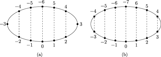
Figure 1. Illustration of the equivalence classes defined by (22) with d = 1. (a) Equivalence classes, ![$[x]_{L-1}$](https://content.cld.iop.org/journals/1742-5468/2024/2/023203/revision1/jstatad13fbieqn181.gif) , on
, on  with L = 7. (b) Equivalence classes,
 ![$[x]_{L}$](https://content.cld.iop.org/journals/1742-5468/2024/2/023203/revision1/jstatad13fbieqn183.gif) , on
, on  with L = 7. Note that in both cases the set of equivalence classes are in bijection with
  .
.
Download figure:
Standard image High-resolution imageThe proof of lemma 3.1, which is based on Markov chain projection arguments, is discussed in section 7.
3.2. Main results for RLRW two-point functions
We now state our main results for the asymptotic behaviour of RLRW two-point functions on  , for periodic, reflecting and holding boundary conditions. We defer proof of these results to sections 5 and 6. We provide numerical evidence of the connection of these results to the Ising and SAW models in section 4.2.
The RLRW model on  is most easily understood by relating it to the RLRW on the infinite lattice. The asymptotic behaviour of the latter was studied in detail in [24]. See also [25].
Suppose  is chosen so that its typical scale aL
grows with L. One would expect the behaviour of
is chosen so that its typical scale aL
grows with L. One would expect the behaviour of  to differ qualitatively depending on whether or not aL
grows fast enough that the RLRW can explore distances from the origin of order L, so that the presence of the boundary can be felt. We therefore present two separate results relating
to differ qualitatively depending on whether or not aL
grows fast enough that the RLRW can explore distances from the origin of order L, so that the presence of the boundary can be felt. We therefore present two separate results relating  to
to  , depending on the asymptotics of
  .
.
Let Δ denote the standard degenerate distribution function, i.e. Δ is the indicator function for  .
.
Proposition 3.2. Consider a sequence of  -valued random variables
  , for which there exists a sequence
  satisfying:
- (i).
- (ii) for some λ < 2.
- (iii)There exists such that for all L.
- (iv)There exists a distribution function such that .


Fix  , and let
  be a sequence in
  satisfying
  and
and  . Then, with
  denoting
  ,
,  or
or  , as
, as  we have:

The assumptions on  given in proposition 3.2 imply that typical
  will have length of order
  with λ < 2. Since a simple random walk of length N typically explores distances from the origin of order
  , it then follows that a typical such RLRW will explore distances of order o(L) from the origin, and will therefore be too short to feel the boundary. It is therefore unsurprising that the finite-box and infinite lattice two-point functions are asymptotic on such a scale, for any of the three choices of boundary conditions studied. The spatial scales probed by proposition 3.2 correspond to distances of the order of
  , where aL
is the typical scale of
, where aL
is the typical scale of  . Under the assumptions of proposition 3.2, it follows from proposition 3.2 and [24, proposition 3.1] that

We note that, in particular, if G corresponds to the distribution function of a mean-1 exponential random variable, then we have

with
and where  denotes the modified Bessel function of the second kind [39]. As discussed in [25],
  is intimately related to the Green function of the continuum Laplacian on
  . As elaborated on in section 4, the exponential choice for G here is motivated by the behaviour of the SAW on the complete graph.
We now turn our attention to the case that  .
.
Proposition 3.3. Fix  , and let
  be a sequence in
  satisfying
  . Let
. Let  be a sequence of
  -valued random variables. Let
  denote
  ,
,  or
or  . Then as
  we have:
- (i)If, then
- (ii)If, then


A similar result is given in [18, theorem 1.4] for the case of a geometric walk length distribution, giving upper and lower bounds for the difference between the torus and infinite lattice two-point functions in terms of the susceptibility, but without control of the constants, and with a lower bound that is weaker by a logarithmic factor when d = 4.
Suppose that  is such that
  converges in distribution, and that the limiting distribution function is continuous at the origin. For example, this occurs if
  in either the critical window or the high-temperature scaling window. Now suppose that
  with λ > 2. It then follows
4
from [24, proposition 3.1] that for any sequence
with λ > 2. It then follows
4
from [24, proposition 3.1] that for any sequence  satisfying
  and
and  we have

Therefore, the exponential decay displayed by (24) for λ < 2 cannot be observed when λ > 2. Consequently, proposition 3.3 implies that  decays as a power-law for
  , but is then dominated by a term of order
  for
for  . We note that the scale
  is o(L), and therefore realisable inside
  , iff λ > 2. To probe the crossover from power-law to plateau behaviour we choose
  such that
  for
for  to obtain

4. Numerical results
4.1. Universal walk length distributions
Figure 2(a) shows the simulated results for  and
and  at fugacity
  with
with  . If the boundary of the critical windows for the SAW and Ising model on
  occurs at the square root of the volume, as occurs for the complete graph SAW, then for d = 5 the value
  should lie inside the critical window while
  should lie outside the critical window. Figure 2(a) is clearly consistent with the conjecture that
  and
and  scale like Lλ
when
scale like Lλ
when  , but like
  for
for  . Likewise, the results in figure 2(b) are consistent with the conjecture that
  and
and  scale like
  when
when  , but like Ld
for
, but like Ld
for  . This behaviour is precisely analogous to the complete graph SAW behaviour shown in equations (12) and (13).

Figure 2. Simulated mean and variance of the Ising (rhombi) and SAW (squares) walk lengths on five-dimensional tori. (a) Simulated  and
and  at fugacity
  with
with  , on a log–log scale. The dashed curves passing through the
  data have slope λ, while the curve passing through the λ = 3 data has slope
  . (b) Simulated
  and
and  at fugacity
  with
with  . The dashed curves passing through the
  data have slope 2λ, while the curve passing through the λ = 3 data has slope d.
Download figure:
Standard image High-resolution imageSimilarly, figure 3 illustrates the appropriately scaled/standardised distribution functions of  and
and  for λ = 1 and λ = 3. Figure 3(a) strongly suggests for λ = 1 that
  and
and  converge in distribution to a mean-1 exponential random variable, precisely as stated in equation (14) for the complete graph SAW in the high-temperature scaling window. Likewise, figure 3(b) strongly suggests for λ = 3 that
  and
and  converge in distribution to a standardised half-normal distribution, precisely as stated in equation (15) for the complete graph SAW in the critical window.

Figure 3. (a) Tail of the simulated distribution function,  , of the rescaled SAW length,
  , and rescaled Ising walk length,
  , on five-dimensional tori at fugacity
  with λ = 1. The dashed curve is
  , the tail of the mean-1 exponential distribution. (b) Simulated distribution function,
  , of the standardised SAW length,
  , and standardised Ising walk length,
  , on five-dimensional tori, at fugacity
  and λ = 3. The dashed curve corresponds to the standardised half-normal distribution function, F, given in equation (16).
Download figure:
Standard image High-resolution imageWe note that the same critical window behaviour for the Ising and SAW mean, variance and limit distribution were observed at the estimated infinite-volume critical fugacity,  , on five-dimensional tori in [24]. One can formally view this case as
  .
.
To support the claim that the boundary of the critical window lies at  , table 1 provides estimates of the scaling exponent µ obtained by fitting
  and
and  to an ansatz
  , for various values of λ. As expected from the complete graph SAW results, we indeed observe that
  for each
  , but
, but  for all
  .
.
Table 1. Estimated µ values for  and
and  on
on  with d = 5 at fugacity
  at various values of λ.
| λ |

|

|
|---|---|---|
| 1 | 1.00(1) | 0.998(2) |

| 1.53(5) | 1.499(2) |
| 2 | 2.01(9) | 2.01(1) |

| 2.26(8) | 2.28(6) |

| 2.50(5) | 2.46(4) |
| 3 | 2.51(2) | 2.5(1) |
Based on the above observations, we conjecture that the following holds for any  and
and  . If
. If  and a > 0 then

and there exist constants  such that

and

While if  , then for any

and there exist constants  such that

and

4.2. Universal two-point functions
We now provide numerical evidence that in both the high-temperature scaling window and the critical window, the two-point functions of the SAW and Ising model display the same asymptotic behaviour as does a RLRW whose walk length distribution is chosen to be that of a corresponding complete graph SAW.
We first consider the high-temperature scaling window with λ < 2. Assuming the validity of the conjectures on  and
and  outlined in equations (28) and (29), it follows from standard convergence of types arguments (see e.g. [40, p 193]) that for all

Now let  ,
,  and for fixed
  let xL
satisfy
let xL
satisfy  . Assuming the validity of equation (34), and that the assumptions of proposition 3.2 hold for this choice of
  , it follows from equation (24) that as

Universality then makes it natural to conjecture that the asymptotics of  for the SAW and Ising model on the torus should be given by

for suitable values of the model-dependent constants,  , depending on d, λ and a. Figures 4(a) and (b) provide strong evidence in favour of these conjectures. In figure 4(a), the constants for the SAW are set to α = 0.75,
  , while in figure 4(b) the constants for the Ising model are set to α = 0.75,
  , where
  and
and  were estimated by fitting the mean walk length; see equation (29).

Figure 4. (a) Two-point functions on five-dimensional tori of SAW at fugacity  and λ = 1. The dashed curve corresponds to the ansatz given by equations (36) and (25), with constants
  set to the values described in the text, with
  estimated via simulation. (b) Analogous plot to (a) for Ising case. (c) Two-point functions on five-dimensional tori of SAW at fugacity
  and
and  . The dashed curve corresponds to the plateau ansatz given by equation (38), with constants
  set to the values described in the text, with
  and
and  estimated via simulation. (d) Analogous plot to (c), with λ = 3.
Download figure:
Standard image High-resolution image
We now consider λ > 2. Assuming the validity of the conjecture given by equation (29), the discussion in section 3.2 suggests that we should observe a plateau in this case. Moreover, we expect the order of the plateau to be  for
for  and
and  for
for  . More concretely, suppose
  and let
  , and for fixed
  let xL
satisfy
let xL
satisfy  . Assuming the validity of the conjecture given by equation (29), it follows from proposition 3.3 and equation (26) that

Universality then makes it natural to conjecture that for both the SAW and Ising model on the torus

for suitable model-dependent parameters  , depending on
  and a. Figure 4(c) plots the SAW and Ising cases on tori with d = 5,
  and
and  , with the constants set to α = 0.76 and
  for SAW and α = 0.79 and
  for the Ising model.
Finally, we consider the case  , which lies inside the critical window. Let
  , and for fixed
  let xL
satisfy
let xL
satisfy  . Then assuming the validity of the conjecture given by equation (29), it follows that equation (38) should hold for suitable model-dependent parameters
  , depending on d. Figure 4(d) plots the SAW and Ising cases on tori with d = 5, λ = 3 and
  , with the constants set to α = 0.74 and
  for SAW, and α = 0.71 and
  for the Ising model.
5. Proof of proposition 3.2
Let  be a simple random walk on
  , starting from the origin, and let

We say that  and
and  have the same parity, and write
  , iff
, iff  is even, where
  denotes the
  norm on
  . Clearly,
  if
if  . Rearranging equation (20) we obtain

The proof of proposition 3.2 will utilise the following three lemmas, whose proofs are deferred until the end of this section.
Lemma 5.1. Let  . Then for all
  and all
Lemma 5.2. Let L and d be positive integers. For all  and all
 ![$x\in [-L/2,L/2]^d$](https://content.cld.iop.org/journals/1742-5468/2024/2/023203/revision1/jstatad13fbieqn386.gif)

Lemma 5.3. Consider  -valued random variables
  for which there exists
  satisfying
  and a distribution function
  such that
  . Let
. Let  be a sequence in
  satisfying
  and
and  . Then
Proof of proposition 3.2. Let  be a sequence in
  satisfying
  . In all that follows, any reference to reflecting or holding boundary conditions on
  assumes L is odd.
First note that lemma 3.1 implies

with  . It therefore suffices to show that the left-hand side of equation (42) is o(1) as
  .
.
We first consider the case of periodic boundary conditions. Part (i) of lemma 3.1 implies

and since  for z ≠ 0, equation (40) gives

We begin by showing that the second term on the right-hand side of equation (44) is exponentially small in L. First consider the large n terms. Combining assumption (iii) with the Chernoff bound implies that  . Letting
  , and recalling assumption (ii), it then follows that for any
  we have

for some κ > 0 which depends on d and on the specific sequence of distributions corresponding to  .
.
Now consider the small n terms. Fix c > 0 and let  satisfy
  . Lemma 5.1 implies
But lemma 5.2 implies  for all
  and
and  , and so equation (46) implies
Therefore combining equations (45) and (47) with equation (44) shows that

We now prove an analogous result for reflecting/holding boundaries. From parts (ii) and (iii) of lemma 3.1, we have for 
where  if
if  , and
, and  if
if  . The second and third terms on the right-hand side in equation (49) can be shown to be exponentially small by arguing analogously to the periodic case. Indeed, applying equation (45) immediately shows that
Now, ![$[x_L]_{\tilde{L}}$](https://content.cld.iop.org/journals/1742-5468/2024/2/023203/revision1/jstatad13fbieqn418.gif) is a subset of
is a subset of  of fixed cardinality, 2d
, and so arguing analogously to (47) implies
of fixed cardinality, 2d
, and so arguing analogously to (47) implies

Similarly, since  for all
 ![$y\in[x_L]_{\tilde{L}}\setminus x_L$](https://content.cld.iop.org/journals/1742-5468/2024/2/023203/revision1/jstatad13fbieqn421.gif) , it follows immediately from equation (46) that
, it follows immediately from equation (46) that

Summarising then, we have for  that
that

But lemma 5.3 implies that  , and so it follows from equation (53) that for

□
Proof of lemma 5.1. Let  , and for
 ![$j\in[d]$](https://content.cld.iop.org/journals/1742-5468/2024/2/023203/revision1/jstatad13fbieqn426.gif) let
let  denote the jth coordinate of Sn
. We begin with the elementary observation that if
denote the jth coordinate of Sn
. We begin with the elementary observation that if  for all
 ![$j\in[d]$](https://content.cld.iop.org/journals/1742-5468/2024/2/023203/revision1/jstatad13fbieqn429.gif) then
then ![$\sum_{j\in[d]}(S_n^j)^2\lt a^2$](https://content.cld.iop.org/journals/1742-5468/2024/2/023203/revision1/jstatad13fbieqn430.gif) . It then follows from the union bound that
. It then follows from the union bound that
for any  , where in the last step we utilised the Chernoff bound. Consequently, for any
  we have

A simple calculation shows that for all 

Therefore, taking  we have as
  that
that

The stated result then follows from equation (58) and the specialisation of equation (56) to  . □
. □
Proof of lemma 5.2. First note that  for all
 ![$a\in[-1/2,1/2]$](https://content.cld.iop.org/journals/1742-5468/2024/2/023203/revision1/jstatad13fbieqn438.gif) and
and  . It follows that for any
 ![$x\in[-L/2,L/2]^d$](https://content.cld.iop.org/journals/1742-5468/2024/2/023203/revision1/jstatad13fbieqn440.gif) and
and 
which establishes the lower bound in equation (41).
Now, since  , the Cauchy–Schwarz inequality implies

Since  , we have

This establishes the upper bound in equation (41). □
Proof of lemma 5.3. Since  and
and  , there must exist s > 0 such that
  . It then follows that there exists ε < 1 and
  such that G is continuous at α and
  , which implies

Therefore there exists α > 0 and  < 1 such that for all sufficiently large L

Now let  . Then
  for all sufficiently large L, and

By construction,  and
and  as
as  , and so it follows from [41, theorem 1.2.1, (1.10)] that there exists
  such that for all sufficiently large L

But ![$|x_L|^2/m_L = (\xi^2/\alpha)[1+o(1)]$](https://content.cld.iop.org/journals/1742-5468/2024/2/023203/revision1/jstatad13fbieqn455.gif) and so
and so

Combining equation (65) with equation (63) then yields the stated result. □
6. Proof of proposition 3.3
For integer  , let
, let

The local central limit theorem for simple random walk approximates pn
via  .
.
We will make use of the following lemma, whose proof is deferred to the end of this section. Let

denote the (upper) incomplete gamma function, and let

denote the complementary error function.
Lemma 6.1. Let  be an integer, let a > 0 and let
  . Then,

and there exist  such that

Proof of proposition 3.3. Rearranging equation (44) yields

where


Similarly, rearranging equation (49) yields, for  and with
  if
if  and
and  if
if  ,
,
where


It is convenient in what follows to define the sequence lL via
and to then let yL
denote an arbitrary sequence in  satisfying
  . With this notation, we introduce the abbreviations

The first task is to show that E(L),  , F(L) and
  are all
  . We begin by considering E(L) and
  . Since
  , for any
via a change of variables  in the first sum. Similarly, changing variables in the second sum yields
It then follows that

Now define  ; the motivation for this will become clear following equation (91). We first consider the small n terms in equations (83) and (84). Let
  , with
  . If
. If  then for all
  we have

with  . The triangle inequality then implies that

Since  for all
 ![$y\in[x_L]_{\tilde{L}}\setminus x_L$](https://content.cld.iop.org/journals/1742-5468/2024/2/023203/revision1/jstatad13fbieqn482.gif) and
and  , and since
 ![$[x_L]_{\tilde{L}}$](https://content.cld.iop.org/journals/1742-5468/2024/2/023203/revision1/jstatad13fbieqn484.gif) has only 2d
terms, it immediately follows from equation (86) with z = 1 that we can bound the small n terms in equation (84) via
has only 2d
terms, it immediately follows from equation (86) with z = 1 that we can bound the small n terms in equation (84) via

But since  for any
  , we have that

Therefore, combining the fact that lemma 5.2 implies  , with equations (86) and (88), it then follows that
We therefore see that the sums of the small n terms in E(L) and  are exponentially small in L.
We now consider the large n terms in equations (83) and (84). An elementary argument shows that there exists  such that for any
  and
and 

Using Markov's inequality, it then follows that for any 
Since  is summable over
  , combining equations (89), (87) and (91) shows that

The bounds for F(L) and  are obtained similarly, with the aid of the local central limit theorem. If
  and
and  satisfy
  , then it follows from [26, proposition 2.1.2] that

for some  . It then follows from equations (93), (85) and the triangle inequality that

Just as equations (87) and (89) were obtained from equations (86) and (88), analogous arguments using equation (94) yield

and
The local central limit theorem for the simple random walk (see e.g. [41, theorem 1.2.1]) implies that that for all 

Arguing as in equation (91), and combining with equation (95) and (96) then yields

Next we consider B(L). Let aL
be a positive sequence. For any  we have
If now  , then since
  for all
  , taking
  we have

and therefore

Consequently, if  then choosing
  in equations (99) and (101) implies

while if  then choosing
  with
with  implies

It now remains to study the asymptotic behaviour of A(L). We first consider part (i), and therefore assume  . It follows from lemma 5.2 and equation (70) of lemma 6.1 that

Since  , there exists γ > 0 such that
  for all sufficiently large L. It follows again from lemma 5.2 and equation (70) of lemma 6.1 that


It follows in particular that

Together with equations (102), (92), (98), (71) and (75) this establishes part (i).
We now focus on part (ii), and therefore assume  . Let
. Let  be a sequence satisfying
  and
and  . From lemma 5.2 and equation (70) of lemma 6.1 we have
But equation (69) of lemma 6.1 implies
and, since  is decreasing and continuous and
  ,
,
But, by assumption on aL ,

and so

Combining equations (110) and (114) we then have

In particular, for periodic boundary conditions we have  and so equation (115) implies

while for reflecting or holding boundary conditions we have  and so equation (115) implies

Together with equations (103), (92), (98), (71) and (75) this establishes part (ii). □
Proof of lemma 6.1. Let  . For any
  we have
  for all
 ![$t\in [z-1/2,z+1/2]$](https://content.cld.iop.org/journals/1742-5468/2024/2/023203/revision1/jstatad13fbieqn525.gif) , and so
, and so

A similar argument also produces the lower bound

Now let  , and define
  . Since
  is a bijection of
  , we have

It follows from equations (118) and (119) that

Equation (69) then follows by observing that

We now consider equation (70). Let  and
and ![$\mathbb{A}_n = [-n, n]^d \cap \mathbb{Z}^d$](https://content.cld.iop.org/journals/1742-5468/2024/2/023203/revision1/jstatad13fbieqn531.gif) . Let
. Let  be the set of vertices on the surface of the box
  . Since
  , it follows that

Therefore there exist  such that for all

Now observe that if  denotes the sup norm on
  , then
  and
and  . Consequently,
A lower bound is obtained similarly:
□
7. Proof of lemma 3.1
Let  be a Markov chain on a countable set S with transition matrix P. Let
  be an
be an  -valued random variable, independent of
  . If
. If  for some fixed
  , then we define the corresponding two-point function to be

the expected number of visits to  by time
  .
.
Now let ∼ denote an equivalence relation on S. For each  , we let
 ![$[x]: = \{x^{^{\prime}}\in S: x^{^{\prime}} \sim x \}$](https://content.cld.iop.org/journals/1742-5468/2024/2/023203/revision1/jstatad13fbieqn550.gif) denote its equivalence class, and denote the set of all equivalence classes on S by
denote its equivalence class, and denote the set of all equivalence classes on S by ![$S^{\#}: = \{[x]: x\in S \}$](https://content.cld.iop.org/journals/1742-5468/2024/2/023203/revision1/jstatad13fbieqn551.gif) . For each
. For each  define

We say P respects ∼ if ![$P(x,[y]) = P(x^{{\prime}},[y])$](https://content.cld.iop.org/journals/1742-5468/2024/2/023203/revision1/jstatad13fbieqn553.gif) for all
for all  and all
  . If P respects ∼, it is straightforward to show that the matrix
  on
on  defined by

is stochastic, and that the process ![$([X_t])_{t\in\mathbb{N}}$](https://content.cld.iop.org/journals/1742-5468/2024/2/023203/revision1/jstatad13fbieqn558.gif) is a Markov chain on
is a Markov chain on  with transition matrix
  . See, for example, [42, section 2.3.1].
Lemma 7.1. Let S be a countable set, endowed with an equivalence relation respected by the stochastic matrix P. Let  be a Markov chain with transition matrix P, and let
  be an
be an  -valued random variable, independent of
  . Let g be the corresponding two-point function of
  , and
, and  be the corresponding two-point function of
 ![$([X_t])_{t\in\mathbb{N}}$](https://content.cld.iop.org/journals/1742-5468/2024/2/023203/revision1/jstatad13fbieqn567.gif) . Then for
. Then for ![$[x],[y]\in S^\#$](https://content.cld.iop.org/journals/1742-5468/2024/2/023203/revision1/jstatad13fbieqn568.gif) and all
and all ![$x^{^{\prime}}\in[x]$](https://content.cld.iop.org/journals/1742-5468/2024/2/023203/revision1/jstatad13fbieqn569.gif) we have
we have
Proof. Let  . A simple induction on t shows that
 ![$(P^{{\#}})^t([x],[y]) = P^{t}(x^{{\prime}},[y])$](https://content.cld.iop.org/journals/1742-5468/2024/2/023203/revision1/jstatad13fbieqn571.gif) for all integers
for all integers  and all
 ![$x^{{\prime}}\in [x]$](https://content.cld.iop.org/journals/1742-5468/2024/2/023203/revision1/jstatad13fbieqn573.gif) . Therefore if
. Therefore if ![$x^{\prime} \in [x]$](https://content.cld.iop.org/journals/1742-5468/2024/2/023203/revision1/jstatad13fbieqn574.gif) , it follows that
, it follows that
□
7.1. Proof of lemma 3.1
The proof of lemma 3.1 relies on the following two results, whose proofs are deferred to section 7.2. Recall the definition of ![$[x]_L$](https://content.cld.iop.org/journals/1742-5468/2024/2/023203/revision1/jstatad13fbieqn575.gif) given in equation (22).
given in equation (22).
Lemma 7.2. Let  , and let
  denote the transition matrix of the simple random walk on
  with periodic boundary conditions. If
  , then for all
 ![$x^{\prime}\in[x]_L$](https://content.cld.iop.org/journals/1742-5468/2024/2/023203/revision1/jstatad13fbieqn580.gif)

Lemma 7.3. Let  , and let
  ,
,  , and
, and  denote the transition matrices of the simple random walk on
  with periodic, holding and reflective boundary conditions, respectively. For any odd L we have


for all  .
.
Proof of lemma 3.1. Let P denote the transition matrix of the simple random walk on  , and let
  denote the transition matrix of the simple random walk on
  with
with  boundary conditions, where
  can denote
  ,
,  or
or  , for periodic, reflecting or holding, respectively. Fix a random variable
  , and let g denote the two-point function defined in equation (127) corresponding to P and
  . Likewise, let
  denote the two-point function corresponding to
  and
and  . The corresponding two-point functions defined in section 3 are the specialisations of g and
  to the case
  . We therefore freely omit the first argument of equation (127) when convenient, with the understanding that in such instances it takes the value 0.
We begin by proving part (i). Consider the equivalence relation on  defined so that to each
  there corresponds the equivalence class

It is straightforward to verify that P respects this equivalence relation, and a simple calculation shows that ![$P^\#([x],[y]) = P_{\mathrm{P},L}(x,y)$](https://content.cld.iop.org/journals/1742-5468/2024/2/023203/revision1/jstatad13fbieqn604.gif) for all
for all  . We therefore have for any
  that
that
where the penultimate step follows from lemma 7.1. This establishes part (i).
Similarly, since  we have for all
  that
that
where the second step follows from lemmas 7.2 and 7.3, and the last step follows from lemma 7.1. This establishes part (ii). Part (iii) is proved similarly. □
7.2. Proof of lemmas 7.2 and 7.3
Recall the definition of ![$[x]_L$](https://content.cld.iop.org/journals/1742-5468/2024/2/023203/revision1/jstatad13fbieqn609.gif) given in equation (22). If
given in equation (22). If  and
and ![$i\in[d]$](https://content.cld.iop.org/journals/1742-5468/2024/2/023203/revision1/jstatad13fbieqn611.gif) , we will write
, we will write  iff
iff  , where we emphasise that addition and multiplication are modulo 2L. If
  for all
 ![$i\in[d]$](https://content.cld.iop.org/journals/1742-5468/2024/2/023203/revision1/jstatad13fbieqn615.gif) , then we will also write
, then we will also write  , so that
  iff
iff ![$y\in[x]_L$](https://content.cld.iop.org/journals/1742-5468/2024/2/023203/revision1/jstatad13fbieqn618.gif) . To avoid confusion, in this section we will denote adjacency between two vertices
. To avoid confusion, in this section we will denote adjacency between two vertices  by
by  , where the value of L will be clear from the context.
Proof of lemma 7.2. A simple random walk on  with periodic boundary conditions corresponds to a simple random walk on
  . Let
. Let  . Then

where  is the set of neighbours of x in
  .
.
Let  . Suppose
 ![$N(x^{^{\prime}})\cap[y]_L$](https://content.cld.iop.org/journals/1742-5468/2024/2/023203/revision1/jstatad13fbieqn627.gif) is nonempty, and let
is nonempty, and let ![$z^{^{\prime}} \in N(x^{^{\prime}}) \cap [y]_L$](https://content.cld.iop.org/journals/1742-5468/2024/2/023203/revision1/jstatad13fbieqn628.gif) . Then
. Then  for some
  and
and  , where ek
denotes the standard unit vector along the kth coordinate axis. Consider
, where ek
denotes the standard unit vector along the kth coordinate axis. Consider

Clearly,  . Moreover, for all i ≠ k we have
  since
since ![$z^{^{\prime}} \in [y]_L$](https://content.cld.iop.org/journals/1742-5468/2024/2/023203/revision1/jstatad13fbieqn634.gif) , so that
, so that  . Furthermore, if
  then
then  , while if
  then
then  , so that in either case
  . It then follows that
  and so
 ![$z \in N(x) \cap [y]_L$](https://content.cld.iop.org/journals/1742-5468/2024/2/023203/revision1/jstatad13fbieqn642.gif) . In particular, we see that
. In particular, we see that ![$N(x^{^{\prime}})\cap[y]_L$](https://content.cld.iop.org/journals/1742-5468/2024/2/023203/revision1/jstatad13fbieqn643.gif) is nonempty iff
is nonempty iff ![$N(x)\cap[y]_L$](https://content.cld.iop.org/journals/1742-5468/2024/2/023203/revision1/jstatad13fbieqn644.gif) is nonempty.
is nonempty.
Suppose now that ![$N(x)\cap[y]_L$](https://content.cld.iop.org/journals/1742-5468/2024/2/023203/revision1/jstatad13fbieqn645.gif) is nonempty, and define
is nonempty, and define ![$f:N(x)\cap[y]_L\to N(x^{^{\prime}})\cap[y]_L$](https://content.cld.iop.org/journals/1742-5468/2024/2/023203/revision1/jstatad13fbieqn646.gif) via
via

The above argument implies that for any ![$z^{^{\prime}} = x^{^{\prime}}+\delta e^k\in N(x^{^{\prime}})\cap[y]_L$](https://content.cld.iop.org/journals/1742-5468/2024/2/023203/revision1/jstatad13fbieqn647.gif) , if we define
, if we define ![$z\in N(x)\cap[y]_L$](https://content.cld.iop.org/journals/1742-5468/2024/2/023203/revision1/jstatad13fbieqn648.gif) as in equation (137) then
as in equation (137) then
and so f is surjective.
Now suppose ![$z,z^{^{\prime}} \in N(x) \cap [y]_L$](https://content.cld.iop.org/journals/1742-5468/2024/2/023203/revision1/jstatad13fbieqn649.gif) satisfy
satisfy  . Without loss of generality, suppose
  , so that

If  with
with  , then
  . So
. So  implies
  , and it follows that

and  implies
  . Therefore,
  , which implies f is injective. We conclude that since f bijective,
 ![$|N(x) \cap [y]_L| = |N(x^{^{\prime}}) \cap [y]_L|$](https://content.cld.iop.org/journals/1742-5468/2024/2/023203/revision1/jstatad13fbieqn660.gif) for all
for all  and
and ![$x^{^{\prime}}\in[x]_L$](https://content.cld.iop.org/journals/1742-5468/2024/2/023203/revision1/jstatad13fbieqn662.gif) . The stated result then follows from equation (136). □
. The stated result then follows from equation (136). □
Proof of lemma 7.3. Let  and set
  . We first consider equation (131). By construction,
  . Let
. Let  denote the set of equivalence classes on
  defined by equation (22). Since the map
  defined by
 ![$x\mapsto [x]_{2l}$](https://content.cld.iop.org/journals/1742-5468/2024/2/023203/revision1/jstatad13fbieqn669.gif) is a bijection, and since both
is a bijection, and since both  and
and  are stochastic, in order to show that
 ![$P_{\mathrm{R},2l+1}(x, y) = P_{\mathrm{P},4l}^\#([x]_{2l},[y]_{2l})$](https://content.cld.iop.org/journals/1742-5468/2024/2/023203/revision1/jstatad13fbieqn672.gif) for all
for all  , it suffices to consider only pairs
  with
with  . By definition,
  only if
  for some
  and
and ![$k \in [d]$](https://content.cld.iop.org/journals/1742-5468/2024/2/023203/revision1/jstatad13fbieqn679.gif) .
.
Let  with
with  for all
 ![$i \in[d]$](https://content.cld.iop.org/journals/1742-5468/2024/2/023203/revision1/jstatad13fbieqn682.gif) . Suppose
. Suppose  for
for  and
and ![$k\in[d]$](https://content.cld.iop.org/journals/1742-5468/2024/2/023203/revision1/jstatad13fbieqn685.gif) . Clearly,
. Clearly, ![$y \in N(x) \cap [y]_{2l}$](https://content.cld.iop.org/journals/1742-5468/2024/2/023203/revision1/jstatad13fbieqn686.gif) , where N(x) is the set of neighbours of x in
, where N(x) is the set of neighbours of x in  . Suppose
 ![$y^{^{\prime}} \in [y]_{2l}$](https://content.cld.iop.org/journals/1742-5468/2024/2/023203/revision1/jstatad13fbieqn688.gif) . Then either
. Then either  or
or  . Clearly
  , and
, and  iff
iff  , but the latter cannot hold, since the left-hand side is odd, the right-hand side is even, and addition is modulo 4l. We therefore see that
  . In order for yʹ to belong to N(x), it is therefore necessary that
  for all i ≠ k. Defining
  via
via  for i ≠ k and
  we conclude that
 ![$\{y\} \subset N(x) \cap [y]_{2l} \subset \{y,\tilde{y} \}$](https://content.cld.iop.org/journals/1742-5468/2024/2/023203/revision1/jstatad13fbieqn699.gif) . Since
. Since ![$\tilde{y} \in [y]_{2l}$](https://content.cld.iop.org/journals/1742-5468/2024/2/023203/revision1/jstatad13fbieqn700.gif) by construction, we have
by construction, we have

But  if and only if
  for
for  . And
. And  if and only if
  . So
. So ![$|N(x) \cap [y]| = 2$](https://content.cld.iop.org/journals/1742-5468/2024/2/023203/revision1/jstatad13fbieqn706.gif) if and only if
if and only if  , which holds iff
  modulo 4l, which in turn holds iff
  . It follows that if
  then
then
We next consider equation (132). Note that  , and let
  denote the set of equivalence classes on
  corresponding to equation (22). Since the map
  defined by
 ![$x \mapsto [x]_{2l+1}$](https://content.cld.iop.org/journals/1742-5468/2024/2/023203/revision1/jstatad13fbieqn715.gif) is a bijection, arguing as above it suffices to show
is a bijection, arguing as above it suffices to show ![$P_{\mathrm{P},2(2l+1)}^{\#}([x]_{2l+1},[y]_{2l+1}) = P_{\mathrm{H},2l+1}(x,y)$](https://content.cld.iop.org/journals/1742-5468/2024/2/023203/revision1/jstatad13fbieqn716.gif) for all
for all  with
with  . By definition,
  only if
  for some
  and
and ![$k \in[d]$](https://content.cld.iop.org/journals/1742-5468/2024/2/023203/revision1/jstatad13fbieqn722.gif) or if y = x.
or if y = x.
Let  . It is straightforward to show that
  if and only if
  which implies
 ![$|N(x) \cap [x]_{2l+1}| = \sum\nolimits_{i = 1}^d {\unicode{x1D7D9}} \big(|x_i| = l \big)$](https://content.cld.iop.org/journals/1742-5468/2024/2/023203/revision1/jstatad13fbieqn726.gif) , where N(x) is the set of neighbours of x in
, where N(x) is the set of neighbours of x in  , and therefore
Suppose instead that  with
with  . Then
  and so if
 ![$y^{^{\prime}} \in [y]_{2l+1}$](https://content.cld.iop.org/journals/1742-5468/2024/2/023203/revision1/jstatad13fbieqn731.gif) then
then  . If
. If ![$y^{^{\prime}} \in [y]_{2l+1}$](https://content.cld.iop.org/journals/1742-5468/2024/2/023203/revision1/jstatad13fbieqn733.gif) then either
then either  or
or  . But since
  , we have
  for
for  and
and

It follows that  . But in order for
  , it is necessary that
  . So we conclude that if
  then
then  , which then implies that
  . It also then follows that
  for all i ≠ k, so that
  . We have therefore established that
 ![$N(x) \cap [y]_{2l+1} = \{y\}$](https://content.cld.iop.org/journals/1742-5468/2024/2/023203/revision1/jstatad13fbieqn747.gif) when
when  with
with  , and it follows that

□
Acknowledgments
The authors thank Gordon Slade for sharing an earlier version of [18] during the final stages of completion of an earlier version of this work. This research was supported by the Australian Research Council Centre of Excellence for Mathematical and Statistical Frontiers (Project No. CE140100049), and the Australian Research Council's Discovery Projects funding scheme (Project Nos. DP180100613 and DP230102209). It was undertaken with the assistance of resources and services from the National Computational Infrastructure (NCI), which is supported by the Australian Government. Y D was supported by the National Natural Science Foundation of China (under Grant No. 12275263), the Innovation Program for Quantum Science and Technology (under Grant No. 2021ZD0301900), and the Natural Science Foundation of Fujian province of China (under Grant No. 2023J02032).
Footnotes
- 4
Although the statement of [24, proposition 3.1] specifies ξ > 0, its proof also holds when ξ = 0.