


Abstract
To obtain engineering-feasible designs of stellarators with permanent magnets and simplified coils, a new algorithm has been developed based on Fourier decomposition and surface magnetic charges method. The strong toroidal fields in a quasi-axisymmetric stellarator are still generated by coils. The permanent magnets are designed to compensate the normal magnetic field Bn on the plasma surface ∂P created by the coils and plasma. The normal magnetic fields created by the permanent magnets Bpmn are calculated as the difference between the magnetic fields created by the surface magnetic charges on the inner surface ∂D and the outer surface ∂Dh of the magnets. The Fourier coefficients of the magnet thickness function  are computed through matrix division operation based on the least square principle with dominant Fourier components selected through 2D Fourier transformation of Bpmn. The residual uncompensated Bn is minimized through iteration to progressively optimize the thickness function. This new algorithm has been successfully applied to design the permanent magnets of an l = 2 quasi-axisymmetric stellarator with background magnetic field created by 12 identical circular planar coils for demonstrations. High accuracy has been achieved, allowing for a flux-surface-averaged residual Bn relative to the total field
  and a maximum residual Bn of less than 2 Gs for ∼1 T total field. This new design has some advantages in engineering implementations: all permanent magnet pieces have the same remanence Br; only one single layer of magnets are mounted perpendicular to the winding surface; the magnets can be easily inserted into the cells of a gridded frame attached to the winding surface and fixed with springs from the back, which greatly simplifies the manufacture, assembly and maintenance of the magnets, and thus facilitates precision control and cost reduction.
Export citation and abstract BibTeX RIS

Original content from this work may be used under the terms of the Creative Commons Attribution 3.0 licence. Any further distribution of this work must maintain attribution to the author(s) and the title of the work, journal citation and DOI.
1. Introduction
Intrinsically steady-state operation, nearly disruption-free and low recirculating power make stellarator an attractive fusion reactor candidate [1]. Historically, stellarators lagged behind tokamaks due to their relatively poor neoclassical confinement. To improve the neoclassical confinement, quasi-symmetry was introduced into the stellarator optimization and the effect has been demonstrated in the HSX stellarator experiments [2]. Recently, the remarkable success of the W7-X stellarator shows that neoclassical optimization can improve the confinement of stellarators up to a level similar to tokamaks [3]. The conventional stellarators use external coils to produce a non-axisymmetric magnetic field which confines the plasma and create the required rotational transform. The required coils in a stellarator are thus very complicated and contribute significantly to the overall cost of the device [4]. Coil complexity is one of the main challenges for stellarators. Modern stellarators use discrete modular coils instead of continuous coils. Even with optimized modular coils, difficulties in fabrication and assembly of the complex 3D non-planar coils with required accuracy and the anticipated strong mechanical stresses in the coils and the support structure of the coils for a reactor-size device have been the main challenges for the development of the stellarator approach as a fusion reactor candidate [5].
Recent study suggests that permanent magnets can be used to create rotational transform in a stellarator, thus substantially simplifying the coils [6], which may facilitates machine construction and cost reduction. More important, higher field strength can be achieved for a reactor-size stellarator as the mechanical stresses in the coils and the support structure of the coils are reduced. Identical planar coils with circular cross-section have been proven sufficient for a quasi-axisymmetric stellarator, leaving permanent magnets to do most of the plasma shaping. The strong background toroidal magnetic fields in a quasi-axisymmetric stellarator are still generated by coils. The permanent magnets can be used just to compensate the fields perpendicular to the plasma outermost surface, i.e., the last closed flux surface. Therefore, the required field strength created by the permanent magnets is not so strong (typically <0.5 T) for an experimental device without blanket or with a thin blanket (<0.3 m). Such field strength is achievable with commercially available permanent magnets which have a remanence of Br ⩽ 1.55 T [7]. In contrast to coils, permanent magnets can provide a steady magnetic field without energy consumption, be arranged in complicated patterns, and more importantly, the materials are relatively inexpensive compared with superconducting materials, thus may drastically reduce the capital cost of a stellarator. However, compared with superconducting magnets the disadvantage is that the magnetic field strength produced by permanent magnets cannot change once the device has been assembled.
Several algorithms have been proposed recently for the design of permanent magnets and applied to the design of quasi-axisymmetric stellarators with highly simplified coils. One is to design the distribution and orientation of the magnetization M of permanent magnets with a fixed thickness [6]. This work verifies the feasibility of creation of rotational transform in a stellarator using permanent magnets. With spatially varying magnetization, engineering realization is difficult as the magnets need to be magnetized to different remanence, which would dramatically increase the difficulty in magnetization precision control and the manufacturing cost. An improved algorithm, the so-called 'multi-layer method', has been explored, through varying the thickness of permanent magnets perpendicular to the installation surface, i.e., the 'winding surface', with a fixed magnetization M [8]. This algorithm calculates the distribution of one thin layer (1 mm thick) of permanent magnets for each step, and then iterates through incrementally stacking magnets layer by layer from innermost to outermost surface with linear method based on the surface current potential distributions, so that the existing codes for stellarator coil design can be used for the permanent magnet design. The solution with this algorithm provides a good initial guess for further optimizations. Recently, a more sophisticated algorithm has been proposed based on finite elements of discretized magnetic dipole moments [9] using the so-called 'density method' [10] with a penalization technique which employs a continuous exponential function to penalize the intermediate values between 0 and 1 to achieve a polarized distribution of the magnet normalized density ρ. With this algorithm, the restriction on the magnetic-dipole orientations can be relaxed, so that the so-called 'Halbach' arrays [11] are formed and less magnets are used than the linear method. In addition, it allows to reserve space for ports, showing attractively large access on the outboard side. More recently, a preliminary study of geometric concepts for magnet arrays is performed [12]. Two classes of magnet geometry, curved bricks and hexahedra, are explored.
Engineering implementation favors uniform remanence and simple geometry for all magnet pieces and a relatively small number of magnet pieces, to simplify the manufacture, assembly and maintenance of the magnets, and reduce the cost. If each magnet piece is too small, there will be a huge number of pieces, which may lead to assembly errors and accumulated errors in the produced magnetic field. Thus, it is worth seeking more advanced algorithms for engineeringly practical magnet design. In this paper a new algorithm is proposed with fixed remanence Br and varying magnet thickness perpendicular to the installation surface based on Fourier decomposition and surface magnetic charges method, which has been demonstrated to be a very effective algorithm, capable of achieving the design targets with high accuracy and a relatively small number of magnet pieces, thus exhibiting attractive engineering feasibility.
This paper is organized as follows. In section 2, the new algorithm and its design logic are introduced with formulations. In section 3, application of this new algorithm to an l = 2 quasi-axisymmetric stellarator with a β = 0 equilibrium is presented. In section 4, numerical validations with field-line tracing are carried out to check the accuracy of the produced flux surfaces relative to the equilibrium flux surfaces. A summary and discussions for future application and development are presented in the last section.
2. Algorithm
To introduce the new algorithm with illustrations, a β = 0 equilibrium for ESTELL stellarator [13] is used, which is an optimized two-period l = 2 quasi-symmetric stellarator with average major radius of the magnetic axis R0 = 1.3944 m and average field strength on the magnetic axis B0 = 1 T. It was originally obtained by deforming a classical l = 2 stellarator with aspect ratio A = 5 into a shape that makes the magnetic field quasi-axisymmetric. This means that the field strength is nearly independent of the toroidal angle in Boozer or Hamada coordinates, which ensures good orbit confinement [14–16]. Here, β = 0 implies that there is no magnetic field produced by plasma current, Bplasma = 0. Figure 1 shows the permanent magnet distribution designed for this ESTELL equilibrium.

Figure 1. Permanent magnet distribution designed for a two-period l = 2 quasi-axisymmetric stellarator with 120 (poloidal) × 240 (toroidal) pieces mounted on the winding surface ∂D with their magnetic axes perpendicular to this surface. The red flux surfaces show the area of plasma. The colorbar indicates the magnet thickness h, i.e., the distance between ∂D and ∂Dh . Positive value (red) means that the magnetic axis of the permanent magnet points away from the plasma and negative value (blue) means toward the plasma.
Download figure:
Standard image High-resolution imageThe permanent magnets are composed of 120 (poloidal) × 240 (toroidal) small pieces, mounted on the winding surface ∂D with their magnetic axes perpendicular to this surface. ∂D could be the outer surface of the vacuum-chamber wall, which encloses and at a distance d from the plasma surface ∂P. ∂Dh is the outer surface composed by the permanent magnets. This design greatly facilitates engineering assembly. The permanent magnets can be easily inserted into the cells of a gridded frame attached to the winding surface and fixed with springs and caps from the back as shown in figure 2. The distance between the winding surface ∂D and the plasma surface ∂P is d = 10 cm and the maximum magnet thickness is hmax = 17.22 cm in this example.
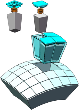
Figure 2. Schematic diagram of the concept for permanent magnet assembly. Magnet pieces are inserted into the cells of a gridded frame attached to the winding surface, fixed with springs and caps from the back.
Download figure:
Standard image High-resolution image2.1. Magnetic field calculation using the surface magnetic charges method
We need to calculate the normal magnetic field component on the plasma surface generated by permanent magnets Bpmn. The magnetic field generated by a piece of permanent magnet is governed by the Biot–Savart law. There are three methods to calculate the magnetic field, i.e., surface magnetic charges, effective currents and discretized magnetic dipoles. The method adopted in this paper is the surface magnetic charges [17], where the permanent magnets are modeled as distributed positive and negative magnetic monopoles with surface charges concentrating on the inner and outer surfaces of the permanent magnets situated 'h' distance apart. The field strength at a field point  on the plasma surface ∂P is a 2D integral across the winding surface ∂D,

Hereafter, primes are used to denote coordinates on the plasma surface and un-primed for the winding surface.
Here, r = x' − x is the position vector pointing from the source point on the winding surface ∂D to the field point and rh
= x' − xh
is the position vector pointing from the source point on the outer surface of the permanent magnets ∂Dh
to the field point.  and
and  are the corresponding distances.
  is the source point on the winding surface ∂D and
  is the source point on the outer surface of the permanent magnets ∂Dh
, which is calculated with the coordinate relationship xh
= x + h
n, where n is the unit normal vector of the winding surface with positive direction pointing outwards (away from the plasma). dΨ = Br± dS is the magnetic flux passing through the inner surface of a magnet piece, i.e., a small quadrilateral on the winding surface. dS is its surface area, which is computed numerically from the coordinates of the quadrilateral's four vertices. Br± is the surface density of the surface magnetic charges. As the magnets are installed perpendicular to the winding surface, Br± is also the normal field produced by the magnets on the winding surface,
is the source point on the outer surface of the permanent magnets ∂Dh
, which is calculated with the coordinate relationship xh
= x + h
n, where n is the unit normal vector of the winding surface with positive direction pointing outwards (away from the plasma). dΨ = Br± dS is the magnetic flux passing through the inner surface of a magnet piece, i.e., a small quadrilateral on the winding surface. dS is its surface area, which is computed numerically from the coordinates of the quadrilateral's four vertices. Br± is the surface density of the surface magnetic charges. As the magnets are installed perpendicular to the winding surface, Br± is also the normal field produced by the magnets on the winding surface,

where  is the sign function. Br± is positive when the magnetization M of the permanent magnet points outwards, i.e., away from the plasma. Its absolute value is equal to the remanence,
  . The remanence varies with materials and material grades. In this paper, we choose Br = 1.4 T for all the calculations, as this is one of the most widely commercially available neodymium–iron–boron (Nd–Fe–B) magnet at room temperature in the market [7]. Note that here it has been assumed that the magnetic flux passing through the outer surface of the permanent magnets is approximately equal to that passing through the inner surface, since there are nearly no gaps between adjacent magnets.
2.2. Design logic
2.2.1. Coil design and optimization target
Most of the magnetic fields in a quasi-axisymmetric stellarator are toroidal magnetic fields which are still produced by coils. Identical circular cross-section planar coils are used to generate the background magnetic field Bcoil (mostly toroidal field) with the minimum field strength (near the outer midplane) equal to that of the equilibrium field strength, Bcoil min = Beq min, to minimize the magnet coverage and offer large access to the plasma on the outboard side, which can be used for heating systems, diagnostics and remote maintenance. The easy access for remote maintenance is extremely favourable for future fusion reactors. The magnetic field component normal to the plasma surface generated by the coils is Bcoiln = Bcoil ⋅ n', where n' is the unit normal vector of the plasma surface with positive direction pointing outwards (away from the plasma). The total equilibrium magnetic field consists of three components, Beq = Bcoil + Bpm + Bplasma. Since there is no magnetic field produced by plasma current in this case, Bplasma = 0, the magnetic field needs to be produced by the permanent magnets is Bpm = Beq − Bcoil.
The permanent magnets are designed to compensate the normal fields produced by the coils and plasma on the plasma surface, Bpmn = Bpm ⋅ n' = −Bcoiln − Bplasman, so as to minimize the surface integral of the residual normal field square, the so-called residual normal field error,

where  is the residual normal field on the plasma surface, which progressively vanishes through iteration, so that
  . Here,
  is produced by the permanent magnets, which approximates the compensation target,
  .
.
Figure 3 outlines the algorithm. After coil design, a database of 2D Fourier base functions is built, as shown in the green part of figure 3, introduced in subsection 2.2.4. The database only needs to be calculated once. Then, iteration starts until a convergence criterion is reached. The iteration flow is shown in the red part of figure 3, which will be introduced step by step in the following subsections.
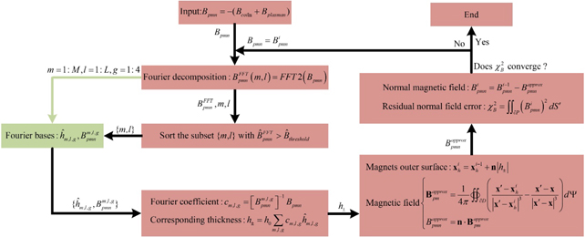
Figure 3. The iteration flow chart of the algorithm. The green part is a database of 2D Fourier base functions, which only needs to be calculated once. The red part is the iteration flow, which uses the database and upgrade the database if additional high-order Fourier base functions are needed.
Download figure:
Standard image High-resolution image2.2.2. 2D Fourier transformation of normal field on the plasma surface
A magnetic-flux coordinate system  is used with grids 120 (poloidal) × 240 (toroidal) × 65 (radial). Here, θ, ϕ and ψ are the poloidal angle, toroidal angle and magnetic flux surface coordinates, respectively. For the flux surface coordinate ψ, the first layer is the magnetic axis and the outermost layer (65) is the plasma surface. Note that some calculations in this algorithm are performed in the Cartesian coordinate system
  . A transformation connects these two coordinate systems.
We find that the normal field  is a 2D continuous function. Its 2D Fourier transformation is calculated,

and normalized to its maximum,  . Here, m is the poloidal mode number and l is the toroidal mode number. Next, a threshold is used to find out the dominant Fourier components,

Only these Fourier components are compensated by the magnetic field generated by the permanent magnets. The other Fourier components are neglected as their amplitudes are small. This spectral truncation method effectively saves computing resources. The NESCOIL code developed by Merkel also uses the spectral truncation method to represent the surface current potential Φ in the design of stellarator coils [18].
2.2.3. 2D Fourier expansion of thickness function on the winding surface
The distributions of magnet thickness and orientation (toward or away from the plasma) on the winding surface are 2D functions,  and
and ![$\mathrm{sign}\left[{B}_{\mathrm{r}{\pm}}\left(\theta ,\phi \right)\right]$](https://content.cld.iop.org/journals/0029-5515/61/2/026025/revision3/nfabcdb6ieqn19.gif) . Here,
. Here,  is the normal field generated by permanent magnets on the winding surface. We introduce a thickness function to describe both the distribution and orientation of the permanent magnets.

Note that  is a signed function. Since in this design the permanent magnets are mounted perpendicular to the winding surface, also nearly perpendicular to the plasma surface, and the winding surface is very close to the plasma surface,
  has a 2D distribution pattern similar to
  . Therefore, the dominant Fourier components in
  are also the ones in
  . The 2D Fourier expansion of
  can be written as,

where h0 = 0.1m is a constant, cm,l,g
are the Fourier coefficients and  are the 2D Fourier base functions. The thickness and orientation can be calculated from
  , i.e.,
  and
and ![${B}_{\mathrm{r}{\pm}}\left(\theta ,\phi \right)={B}_{\mathrm{r}}\enspace \mathrm{sign}\left[{h}_{{\pm}}\left(\theta ,\phi \right)\right]$](https://content.cld.iop.org/journals/0029-5515/61/2/026025/revision3/nfabcdb6ieqn30.gif) .
.
The 2D Fourier base functions  have four kinds of combinations:
  ,
,  ,
,  and
and  . Note that there are some Fourier base functions equal to zero for
  when m = 0 or l = 0. Now, the problem translates into calculating the Fourier coefficients, cm,l,g
. Because of the truncation of Fourier series, the magnetic field will inevitably lose some details with the finite Fourier modes. This is an ill-posed inverse problem, which can be solved using matrix division operation based on the least square principle [19].
when m = 0 or l = 0. Now, the problem translates into calculating the Fourier coefficients, cm,l,g
. Because of the truncation of Fourier series, the magnetic field will inevitably lose some details with the finite Fourier modes. This is an ill-posed inverse problem, which can be solved using matrix division operation based on the least square principle [19].
2.2.4. Build a database of 2D Fourier base functions
The normal fields on the plasma surface  produced by the permanent magnets with each Fourier component of the thickness distribution
  and orientation distribution
 ![${B}_{\mathrm{r}{\pm}}^{m,l,g}\left(\theta ,\phi \right)={B}_{\mathrm{r}}\enspace \mathrm{sign}\left[{\hat{h}}_{m,l,g}\left(\theta ,\phi \right)\right]$](https://content.cld.iop.org/journals/0029-5515/61/2/026025/revision3/nfabcdb6ieqn39.gif) described by the 2D Fourier base functions
described by the 2D Fourier base functions  are calculated in advance, constituting a database for m = 0:M, l = 0:L and g = 1:4. Only nonzero Fourier base functions
  are included in the database. It is found that a database with M = 16 and L = 42 can provide sufficient precision for the following optimization. In the code, for each time iteration, if a Fourier mode outside the database appears, i.e., m > M or l > L, the corresponding data of this Fourier mode, including the normal fields on the plasma surface
  , will be calculated and added into the database to update the database. When the iteration ends, if the database is almost unchanged, which means that most of the Fourier modes involved in the optimization process have been included in the database with the given selection criteria of Fourier mode, the database is considered to be big enough. The magnetic field on the plasma surface
  is calculated using the surface magnetic charges method according to equation (1) with the coordinate relationship
  and the magnetic flux
  . Then, the normal field is obtained,
  .
.
2.2.5. Calculations of Fourier coefficients and residual normal field
For each iteration, the Fourier decomposition is conducted with the updated normal field on the plasma surface. A subset of Fourier modes {m, l, g} is picked out from the database of the 2D Fourier base functions with the selection criteria, in equation (5), and sorted out according to the normalized spectral amplitude. The parameter g = 1:4 corresponds to four kinds of combinations, as given in the last paragraph of section 2.2.3. Then, the Fourier coefficients cm,l,g are calculated through matrix division operation based on the least square principle [19],

where ![${\left[\dots \right]}^{-1}$](https://content.cld.iop.org/journals/0029-5515/61/2/026025/revision3/nfabcdb6ieqn47.gif) is the generalized inverse of a matrix. The magnet thickness function
is the generalized inverse of a matrix. The magnet thickness function  is constructed from the Fourier components by following equation (7). Then, we have the thickness
  and orientation
  . The magnetic field on the plasma surface
  produced by these permanent magnets is calculated using the surface magnetic charges method according to equation (1) with the coordinate relationship
  and magnetic flux
  . Finally, we obtain the approximate normal field on the plasma surface produced by the permanent magnets
  and the residual normal field
  which is the compensation target for the next iteration.
2.2.6. Iteration to progressively correct the thickness function
Iteration starts. The 2D Fourier transformation of  is calculated and the dominant Fourier components is obtained with the same threshold
  . A new subset
  in the database of the 2D Fourier base functions is sorted out according to the dominant Fourier components. Then, a new set of Fourier coefficients are calculated through matrix division operation
 ![${c}_{m,l,g}={\left[{B}_{\text{pmn}}^{m,l,g}\left(\theta ,\phi \right)\right]}^{-1}{B}_{\text{pmn}}^{\text{residual}}\left(\theta ,\phi \right)$](https://content.cld.iop.org/journals/0029-5515/61/2/026025/revision3/nfabcdb6ieqn59.gif) based on the least square principle. With these Fourier coefficients, we obtain a correction to the magnet thickness function
based on the least square principle. With these Fourier coefficients, we obtain a correction to the magnet thickness function  according to equation (7) and a corrected thickness function
  . Note that
  is still a signed function. Again,
  is calculated using the surface magnetic charges method.
  and
and  are obtained as well. Next, we use the residual normal field on the plasma surface
  to calculate the residual normal field error
  according to equation (3). Eventually, the threshold
  is scanned, repeating the iteration, to find out the best threshold with minimum
  . The iteration stops when a convergence criterion is reached, i.e.,
  exceeds the average of the last 5
  values. Then, the iteration with the minimum
  is given as the final result. Under ideal condition,
  will decrease all the way down and never increase between iterations. However, some fine structures associated with the high-order Fourier components of the normal field on the plasma surface are abandoned due to the truncation of the Fourier series. As approaching convergence, the optimization focuses on the fine structures,
  thus fluctuates between iterations. The stopping condition used in this paper is equivalent to the last five-point average of
  over iterations, which is thus insensitive to the fluctuations. Although tolerance can also be used as a stopping condition. However, if the default tolerance cannot be reached, the iteration will be stuck in an endless loop and wastes a lot of machine time. More important, it is difficult to find appropriate tolerances for different cases. The stopping condition used here can be applicable to most cases, provides good results with relatively few iterations and effectively avoids getting stuck in an endless loop.
3. Apply to an l = 2 quasi-axisymmetric stellarator
3.1. Design of the circular planar coils
The first step is to design the coils. Since permanent magnets cannot create toroidal magnetic flux, coils are still necessary to generate a background magnetic field. The strongest magnetic field component in a quasi-axisymmetric stellarator is the toroidal field which is mainly created by coils. However, the utilization of permanent magnets substantially simplifies the coils. Only 12 identical circular cross-section planar coils are used with their coil planes perpendicular to the local magnetic axis, as shown in figure 4, so as to minimize the magnetic field created by permanent magnets, thus minimize the total usage of magnet material. Note that the magnetic axis is a closed 3D curve for a quasi-symmetric stellarator.

Figure 4. (a) The winding surface (blue) of a β = 0 equilibrium for ESTELL, a two-period l = 2 quasi-symmetric stellarator, shown with 12 identical circular cross-section planar coils, all carrying the same current 4.4116 kA. Each coil has 15 × 9 turns. (b) The outer surface of the permanent magnets with color indicating the thickness.
Download figure:
Standard image High-resolution imageThe coil centers have been shifted radially outward in the same coil planes by 0.12 m relative to the local magnetic axis to allow more space on the outboard side for easy access to the plasma and enough gaps between coils on the inboard side to avoid coil interacting with each other. The coil radius is set to 0.9 m to ensure that there is enough space between the coils and the winding surface for the assembly of permanent magnets, see figure 5. The distance between the plasma surface (solid curves) and the winding surface (dashed curves) keeps constant at d = 10 cm.
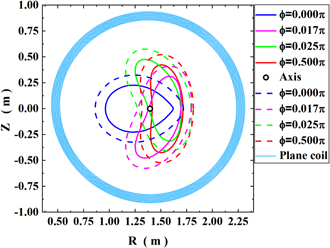
Figure 5. Cross sections of plasma surface (solid curves) and winding surface (dashed curves) at 4 toroidal locations. Projection of the coil at ϕ = 0° (skyblue circles). Toroidally averaged magnetic axis (black hollow dot).
Download figure:
Standard image High-resolution imageEach coil has 15 × 9 turns, carrying the same current Icoil = 4.4116 kA. The magnetic field generated by the coils are calculated by following the Biot–Savart law. The coil current is adjusted to match the minimum magnetic field strength (near the outer midplane) with that of the equilibrium magnetic field, Bcoil min = Bmin = 0.8213 T. The maximum magnetic field on the inboard side is slightly stronger than that of the equilibrium magnetic field, as shown in figures 6(a) and (c). The differences need to be compensated by the magnetic field generated by permanent magnets.

Figure 6. Magnetic fields on the plasma surface, (a) total magnetic field generated by coils Bcoil, (c) total equilibrium magnetic field Beq, (b) 3D plot and (d) contour plot of the normal field produced by the coils Bcoiln.
Download figure:
Standard image High-resolution imageThe 3D plot and contour plot of the normal field produced by the coils Bcoiln are shown in figures 6(b) and (d), respectively. The normal field needs to be produced by the permanent magnets is Bpmn = −Bcoiln. The target is to calculate an approximate normal field  to compensate the normal field produced by the coils Bcoiln on the plasma surface so that
  vanishes.
  appears to be a 2D continuous function. Its largest Fourier component is m, l = 2, 2 mode and l = 12 toroidal ripples can be clearly seen on the outboard side in figures 6(a), (b) and (d).
3.2. 2D Fourier transformation of the normal field on the plasma surface
In order to find out the dominant 2D Fourier components need to be produced by the permanent magnets, 2D Fourier transformation is applied to  . There are many Fourier modes as shown in the 2D spectrum in figure 7(a), however, most of them have very small amplitude. Note that to enhance the spectral visibility natural logarithm has been used in figure 7(a),
  . The dominant Fourier components are sorted out with a normalized-spectral-amplitude threshold,
  . The largest Fourier component appears to be m, l = 2, 2 mode, as shown in figure 7(b).

Figure 7. (a) 2D spectrum of the normal field on the plasma surface with natural logarithm of the normalized amplitude  , (b) 2D spectrum with the normalized amplitude above a threshold
  . In order to reduce computational cost, for those Fourier modes with the same
  and
and  numbers, only one mode is left.
Download figure:
Standard image High-resolution image3.3. Build a database of 2D Fourier base functions
The next step is to build a database of 2D Fourier base functions  and calculate the normal magnet field
  on the plasma surface produced by the permanent magnets described by the Fourier base functions. The largest Fourier component is m, l = 2, 2. The corresponding 2D Fourier base function
  and normal field
  exhibit very similar distribution pattern, see figure 8. The similarity indicates that the Fourier expansion is an effective method in solving the inverse problem of permanent magnet design, similar to the NESCOIL code in designing the stellarator coils. We note that a deviations is visible in the distribution patterns between the two plots in figure 8, i.e., the magnet thickness pattern and the corresponding magnetic field pattern. It is not due to the mismatch in shape between the winding surface ∂D and the plasma surface ∂P, because the winding surface is generated through extending from the plasma surface along its normal vector with a fixed distance d, and thus they have the same shape. If the winding surface and the plasma surface are both planes and parallel to each other, there will be very little deviation. However, they are complicated three-dimensional surfaces with spatially varying surface curvatures. Therefore, the magnetic field pattern will be distorted relative to the magnet thickness pattern.
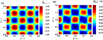
Figure 8. Contour plots of (a) the 2D Fourier base function  for the largest Fourier component m, l = 2, 2 and (b) the normal field on the plasma surface
  produced by the corresponding permanent magnets.
Download figure:
Standard image High-resolution image3.4. Iteration and convergence
Following the calculation steps introduced in section 2.2.5, we truncate a finite number of 2D Fourier components by setting a threshold to the spectral normalized amplitude,  , and calculate the Fourier coefficients cm,l,g
through matrix division operation based on the least square principle. Then, we obtain the approximate normal field on the plasma surface produced by the permanent magnets
, and calculate the Fourier coefficients cm,l,g
through matrix division operation based on the least square principle. Then, we obtain the approximate normal field on the plasma surface produced by the permanent magnets  and the residual normal field
  . At this point, the first design cycle is complete. The initial maximum normal field on the plasma surface produced by the permanent magnets
  (∼1000 Gs) and the residual normal field error
  (∼3 × 10⁻² T2 m2) are still very large. They are effectively reduced through the iterations, as shown in figure 9(b).

Figure 9. (a) Threshold  scan to find out the best threshold with minimum residual normal field error
  , shown in blue. The maximum of residual normal field on the plasma surface
  is shown in red. (b) For the best threshold
  ,
,  (blue) and
  (red) converge to 4.786 × 10⁻⁹ and 1.986 Gs, respectively, after 77 times iterations.
Download figure:
Standard image High-resolution imageFinally, the threshold  is scanned from 0.1 to 0.5 as shown in figure 9(a). The best threshold with minimum residual normal field error
  is found,
  . With this threshold,
  and the maximum of residual normal field on the plasma surface
  converge to 4.786 × 10⁻⁹ and 1.986 Gs, reduced by 7 and 3 orders of magnitude, respectively, after 77 times iterations, as shown in figure 9(b).
The computation was performed using a computer workstation with 48 CPUs at 2.5 GHz. For spatial resolution 120 (poloidal) × 240 (toroidal) grids, each iteration needs roughly 16 min and the threshold scan from 0.1 to 0.5 with step 0.01 totally consumed ∼8.1 h. In addition, the 2D Fourier base function database calculation took ∼7.1 h, which only needs to be computed once.
With the best converged optimization results, the normal field on the plasma surface produced by the permanent magnets  is a very good approximation to the normal field need to be produced by the permanent magnets Bpmn = −Bcoiln, as shown in figures 10(b) and (d). Furthermore, the total magnetic field on the plasma surface produced by the coils and permanent magnets
  is almost identical to the total equilibrium magnetic field
  , as shown in figure 11, which demonstrates the validity of the design algorithm. The residual normal field on the plasma surface
  is less than 2 Gs, see figure 10(c). The most uncompensated Bn
mainly located near the outboard midplane around toroidal angle ϕ = 0 and π, where Bcoiln has a sharp transition between positive and negative as shown in figure 6(b). More high order Fourier components are needed to compensate such sharp transition. This sets the lower limit of field-compensation and design accuracy for the Fourier based method. However, this location can be used to set up a divertor where finite Bn
is favorable. The flux-surface-averaged residual normal fields relative to the total field on the plasma surface is
is less than 2 Gs, see figure 10(c). The most uncompensated Bn
mainly located near the outboard midplane around toroidal angle ϕ = 0 and π, where Bcoiln has a sharp transition between positive and negative as shown in figure 6(b). More high order Fourier components are needed to compensate such sharp transition. This sets the lower limit of field-compensation and design accuracy for the Fourier based method. However, this location can be used to set up a divertor where finite Bn
is favorable. The flux-surface-averaged residual normal fields relative to the total field on the plasma surface is  , exhibiting very high accuracy in the normal field compensation. In addition, the magnet thickness function h± is shown in figure 10(a), which has a 2D distribution pattern very similar to
  , see figure 10(b). This leads us to come up with the idea of Fourier decomposition of the magnet thickness function.
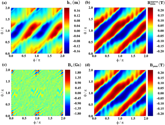
Figure 10. For the best threshold  after convergence, the contour plots of (a) the magnet thickness function h±, (b) the normal field on the plasma surface produced by the permanent magnets
  , (c) the residual normal field on the plasma surface
  and (d) the normal field need to be produced by the permanent magnets Bpmn = −Bcoiln.
Download figure:
Standard image High-resolution image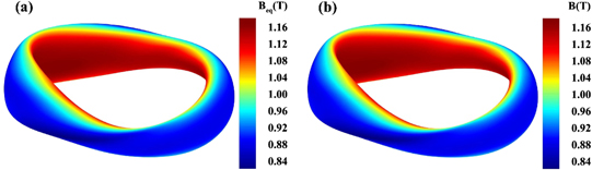
Figure 11. (a) The total equilibrium magnetic field  and (b) the total magnetic field
  produced by the coils and permanent magnets on the plasma surface.
Download figure:
Standard image High-resolution image4. Field line tracing to check the accuracy in generating the target equilibrium
Field-line tracing is calculated to check the accuracy of the produced magnetic flux surfaces relative to the equilibrium magnetic flux surfaces. Since a β = 0 equilibrium has been used, there is no magnetic field produced by plasma current, i.e., Bplasma = 0, the total magnetic field is just the vacuum field, which is produced by the coils and permanent magnets  , and the Shafranov shift is zero as shown in figure 12. The field-line tracing results indicate that the vacuum flux surface fits the target equilibrium magnetic flux surfaces quite well. The relative difference of the rotational transform at the plasma surface (the last closed flux surface) is only Δι/ι = 0.49%, which verifies the validity of the design algorithm.
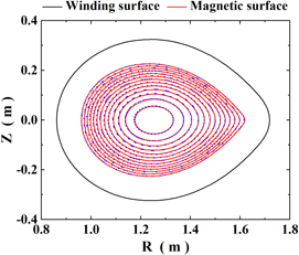
Figure 12. Poincaré plot on the plane at toroidal angle ϕ = 0 from field-line tracing in the magnetic field produced by the coils and permanent magnets  is shown with blue dots. The cross-sections of equilibrium magnetic flux surfaces are shown with red curves. The winding surface is shown with a black curve. The field-line tracing appears to fit the equilibrium magnetic flux surfaces quite well.
Download figure:
Standard image High-resolution imageThe field-line tracing is calculated in the Cartesian coordinate system with an improved six-order Runge–Kutta algorithm [20] following the field-line equation dBx /dx = dBy /dy = dBz /dz. For each point on the tracing trajectory, the magnetic field is calculated based on the Biot–Savart law for the coils and the surface magnetic charges method for the permanent magnets.
5. Discussions and summary
By using permanent magnets, it has been proven possible to build optimized stellarators with extremely simple coils [6, 8, 9]. In this paper, a new algorithm has been proposed for the design of the permanent magnets. It mainly has three new features:
- (a)The surface magnetic charges method [17] has been introduced in this algorithm to calculate the magnetic field produced by the permanent magnets. Compared with other methods, such as the surface-current-potential method [8] and magnetic-dipole-moment method [9], this method is more suitable for the design of permanent magnets with varying thickness.
- (b)The permanent magnets are designed through progressively optimization of the thickness distribution with 2D Fourier decomposition of the thickness function. The Fourier components are selected according to a spectral amplitude truncation of the 2D Fourier transformation of the normal field on the plasma surface.
- (c)To solve the inverse problem, the Fourier coefficients of the magnet thickness function are computed through matrix division operation based on the least square principle [19].
For engineering implementations, this new design algorithm has several advantages:
- (a)All permanent magnet pieces have the same remanence Br, which greatly simplifies the manufacture of the magnets, especially the magnetizing process and precision control. The cost is thus reduced.
- (b)Only one single layer of permanent magnets is installed perpendicular to the winding surface, which greatly simplifies the assembly process and maintenance. The permanent magnets can be easily inserted into the cells of a gridded frame attached to the winding surface and fixed with springs from the back.
- (c)Since there is only one single layer of magnets, for each grid location
 on the winding surface, there is no reversed magnetizations or vacancies in between magnet layers, as in the previous designs [8, 9]. This may reduce the redundancy in the usage of magnet material. To further reduce the total amount of the magnet material usage, relaxing the magnet orientation is required.
 - (d)In this work, a dense mesh (120 × 240) has been used in the computation to improve the field design accuracy. However, this design allows for a much coarser mesh for the magnet distribution during engineering implementation. Since the outer surface ∂Dh of the permanent magnets constitutes a continuous surface, it can be re-divided into a much coarser mesh to reduce the number of magnet pieces and simplify the engineering implementation.
- (e)Although establishment of the 2D Fourier base function database needs a relatively long computational time, it only needs to be computed once. The rest part of the algorithm is rather fast.

Although we have only shown the design results for a quasi-axisymmetric stellarator, the new algorithm can be applied to any configurations. The design solution obtained with this algorithm could be a relatively good initial guess for further nonlinear optimization with more sophisticated codes. For future work, further development in the algorithm is required to relax the constraint on the orientation of the permanent magnets to reduce the total volume of the magnets and allow stay-away zones to incorporate ports. The total volume of magnets used depends on the grids of magnet distribution. Given the same grids, in principle relaxing the constraint on the magnet orientation would allow the total volume of magnets to be reduced, as it would make use of the effect of Halbach array [11]. However, if the grids are different, the result may be opposite. For example, the results of Zhu et al [9] shows that with the same grids, compared with the perpendicular only solution, an orientation-optimized solution uses less magnets. However, with the so-called 'curved bricks' grids, an orientation-optimized solution uses more magnets than the former two solutions. On the other hand, an arbitrary orientation of the magnets would dramatically increase the difficulty and cost of permanent magnet manufacturing.
The feasibility of using permanent magnets in reactor-size stellarators for fusion energy application is still debatable. One should consider the fact that the permanent magnets have to be placed outside the vacuum vessel which will be at least 1 m away from the plasma as there is a breeding blanket in between. To achieve tritium self-sufficiency, a breeding blanket of at least 1 m thick is required [21]. The field strength produced by the permanent magnets on the plasma surface is limited by the maximum achievable remanence Br of the material, which is less than 1.59 T even at liquid nitrogen temperature for currently commercially available magnets such as Pr–Fe–B and Nd–Fe–B [22], except for some special material such as Fe16N2 with Br up to 2.9 T [23]. Although the permanent magnets are used only to compensate the normal field on the plasma surface, which is typically one order of magnitude smaller than the strong background field, it is still very challenging. However, we can use permanent magnets to compensate part of the normal field or produce part of the rotational transform, while we still use 3D modular coils instead of the identical circular planar coils. Even though, the coil complexity can be substantially reduced, which will greatly facilitate the machine construction and cost reduction. Furthermore, higher field strength can be achieved for a reactor-size stellarator as the mechanical stresses in the coils and the support structure of the coils are reduced.
At liquid nitrogen temperature, permanent magnet materials, such as Pr–Fr–B, have a higher remanence Br (up to 1.59 T) and intrinsic coercivity Hcj (larger than 7 T) [22], supposing that the permanent magnets are contained in a cryostat. We note that the demagnetization is mostly effective when the applied background magnetic field is in the opposite direction of the magnet magnetization. However, the projection of the background field in the opposite direction of the magnet magnetization is usually much smaller than the background field for most permanent magnets, especially in an n = 2 quasi-axisymmetric configuration, such as the ESTELL, where the maximum ratio of the projection to the background field is only about 20%. This may imply that the magnets could maintain magnetization in a relatively strong background field. More study is required to clarify this point.
The magnetic field strength produced by permanent magnets appears to be insufficient for a self-sustained fusion reactor. However, it may be sufficient for a fusion neutron source with a neutron wall loading of ⩽0.2 MW m−2, corresponding to a neutron flux rate of ⩽9 × 10¹⁶ m−2 s−1, which only needs a shielding blanket of ⩽0.3 m thick [24]. Furthermore, a big advantage of using permanent magnets relative to copper coils is steady state operation without energy consumption. Compared with superconducting magnets, permanent magnets are much inexpensive. Stellarators with permanent magnets and simple superconducting coils may thus open up a promising new avenue for the development of less-expensive steady-state fusion neutron sources.
Acknowledgments
We would like to acknowledge Michael Drevlak for the ESTELL equilibrium and the helpful communications with Caoxiang Zhu, Haifeng Liu, Samuel Lazerson and Jie Huang. This work was supported by the National Magnetic Confinement Fusion Energy R&D Program of China under Grant No. 2019YFE03030000, the National Natural Science Foundation of China under Grant No. U19A20113, the Key Research Program of Frontier Sciences, CAS under Grant No. QYZDB-SSW-SLH001, the CASHIPS Director's Fund under Grant No. BJPY2019A01 and the K.C. Wong Education Foundation.