


Abstract
The extended-MHD NIMROD code (Sovinec C.R. and King J.R. 2010 J. Comput. Phys. 229 5803) is used to simulate the dynamics of an edge harmonic oscillation (EHO) in quiescent H-mode (QH-mode) DIII-D (Luxon J.L. 2002 Nucl. Fusion 42 614) discharge 163 518. EHOs observed in non-linear MHD simulations have n = 1 and n = 2 as dominant modes akin the DIII-D experiment. Kinetic equilibrium reconstructions during the time of the fully-developed EHO include the effect of the MHD profile relaxation and are found below the stability boundary. This paper discusses methods to include additional instability drives to the experimental equilibria in order to trigger EHO formation. The experimental equilibrium for the DIII-D discharge 163 518 is modified to include two levels of instability drive by increasing the experimental pressure gradient. In order to do a more direct comparison of the simulation results with the experiment, a synthetic BES diagnostic is used to compute cross-correlation and cross-power spectral densities associated with the simulated density perturbations. It is shown that the amplitude of the experimental density perturbations is between the computed density perturbation amplitude for the two levels of instability drive. The synthetic cross-power spectral density shows a transition from a double to a single peak in frequency when the BES analysis shifts from near the LCFS towards the steep gradient region of the pedestal. This observation is similar to the experiment, but the first peak frequency for the weak instability drive is found below the experimental frequencies, and the second peak for the strong instability drive is found above the experimental peak frequencies. However, these peak frequencies are in agreement with the local flow estimate and a MHD turbulence bursty behavior in the simulations with the strong instability drive.
Export citation and abstract BibTeX RIS
1. Introduction
The quiescent H-mode (QH-mode) regime [1–3] is an attractive tokamak operating regime because it has high confinement like H-mode, but avoids the deleterious effects of Edge Localized Modes (ELMs) that normally accompany H-mode. Within this regime, different quiescent dynamics may exist, but they all are characterized by long-wavelength edge activity. There are coherent states featuring the edge harmonic oscillation (EHO) [1–3], and non-coherent regimes, dubbed broadband regimes, that have more turbulent-like states [4, 5].
Next generation tokamaks are challenged by the need to accommodate associated high heat fluxes on the divertor and innovative divertor solutions are being developed. It is critical that these solutions are compatible with edge solutions without ELMs and, given the cost of such devices, predictive simulation is required. Regardless of the different states leading to quiescence, the QH-mode regime is relevant to future burning plasma experiments, such as ITER [4], and thus of extensive interest both computationally [6–9] and theoretically [10, 11].
Prior work with the NIMROD code [8, 9] explains many key features of the broadband regime, including the density pump-out and the critical role of the shear flow. In particular, it is demonstrated that the non-linear simulation with flow yields a saturation state with low-n dominant modes. In the simulation without flows, high-n dynamics dominate and never saturate. In this model, the QH-regime can be viewed as being caused by peeling-ballooning driven turbulence. According to the spectral energy and perturbation dynamics, a weakly turbulent states was observed in the simulation. However, the analysis from local synthetic probes indicated a presence of coherent oscillations. The question if the extended MHD can distinguish the broadband MHD regime from the regime with the edge harmonic oscillations (EHOs) remains. The modeling of QH-mode discharges with EHOs can be considered as a natural extension of the prior work that could potentially address this question. Another question that we want to answer is how do the simulation results depend on the instability drive? Are the final saturated states sensitive to the instability drive? This question is also correlated to the effect of uncertainties in experimental data and fitting procedures. For the simulations with the final saturated states that are sensitive to the initial instability drives, the validation of simulation results becomes especially important. However, the validation of non-linear MHD simulations of edge physics is challenging due to rich physics and competing time scales [13].
In this paper, we show progress in the validation of extended MHD NIMROD [14] simulations in explaining the QH-mode physics of EHOs. The DIII-D discharge 163 518 that has been selected for the analysis in this Paper exhibits a transition between different QH-mode regimes. A spectrogram of the poloidal magnetic field fluctuations is shown in figure 1. All analysis in this manuscript relates to the time slice at t = 2350 ms where an EHO with a dominant n = 1 toroidal mode number is observed. This time slice is marked with a purple vertical line in figure 1. Some basic physics quantities that are used in EFIT reconstuction are shown in figure 2. The DIII-D discharge is well diagnosed and described in a number of previous publications [5, 12, 15, 16].
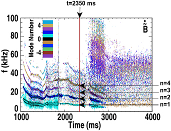
Figure 1. The spectrogram of the poloidal magnetic field fluctuations determined by external magnetic probes. Adapted from [12], with the permission of AIP Publishing.
Download figure:
Standard image High-resolution image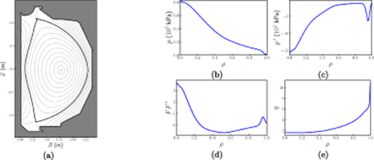
Figure 2. Flux surfaces (a) computed with EFIT for the DIII-D discharge 163 518 at 2350 ms. The total plasma presure (b), presure gradient (c),  (d), and q (e) profiles as functions of normalized toroidal flux.
Download figure:
Standard image High-resolution imageThe general paradigm of simulating QH-mode fusion experiments is that the large gradients required for fusion-relevant densities and temperatures drive instabilities that evolve to a saturated steady-state. This forms the basis of most validation studies using the non-linear extended-MHD and gyrokinetic codes. Fundamentally, the variables to be evolved,  , are decomposed into two parts, an equilibrium part,
  , and a perturbation part,
  . That is, we can write,
  . This decomposition enables one to study the linear stability properties: if the plasma is linearly stable, then the codes do not show growing perturbation. The general procedure for validation of global profiles is thus a linearly unstable equilibrium is generated based on experimental data, the code is run, and then it is validated if the observed profiles match the code profiles:

It is typically assumed that  , but our meaning of
  is specific: it is the Grad-Shafranov solution (force balance) along with the auxiliary profiles (density, ion temperature, electron temperature, etc) that is consistent with that Grad-Shafranov equilibrium. When the perturbations are small, this type of solution, a kinetic EFIT [17] reconstruction is a good approximation and with only slight modifications, often within experimental error bars, can be used in the non-linear codes.
For the large perturbations observed in the edge, both for QH-mode and other regimes, this paradigm is more challenging. The experimental plasma states already include effects resulted from the non-linear physics that the codes are trying to model. That is the difference between  and
and  becomes large enough that the difference lies outside of the measurement error bars, and only relying on slight variations to the equilibrium reconstruction becomes insufficient. To solve this requires a parameter scan, and the larger the perturbation amplitudes under investigation, the more difficult it is to determine the equilibrium. Indeed, observations of QH-mode often show localized flattening expected of instability relaxations [4]. In fact, as diagnostics improve the difference between
  and
and  , the equilibrium that gives rise to the appropriate instability, actually becomes larger, or at least the error bars smaller.
This method can heuristically, and more concretely, be explained in terms of the peeling-ballooning diagram [10, 18] that has been successfully used to explain the general features of edge instabilities. In figure 3, we show how the experimental reconstructions,  for QH-mode are often measured in the stable region, even accounting for experimental uncertainties. We have to go outside of the experimental error bars and develop a new equilibrium that is linearly unstable. For the cases discussed in this paper, we steepen the pressure gradient, and the current by extension due to the bootstrap current, to create cases that are linearly unstable and thus suitable for non-linear simulations. In two linear unstable cases considered in this research, the pressure gradient is increased by factors of 1.4 and 2. Of course, even within the limited parameter space of the peeling-ballooning model, considerable freedom exists in moving from the stable region to the unstable region.
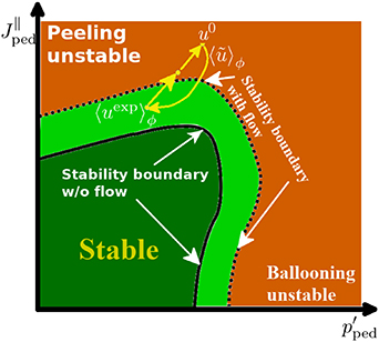
Figure 3. Schematic based on reference [10] of peeling-ballooning instability diagram shows method in creating cases used in this paper. The experimental observations ( ) are in the stable region. Two cases are created by increasing the pedestal gradient, which also increases the current in the edge through the bootstrap current, and creating equilibria that are in the unstable region. The modifications due to flow, and other non-ideal effects, are meant to be heuristic.
Download figure:
Standard image High-resolution imageOur goal is to understand the validation of the resistive MHD model, but this necessarily requires an understanding of the uncertainty of our overall method of simulation and not only the model; specifically how we determine the unstable equilibrium and what we learn from the evolution of the perturbations trying to relax the profiles to the experimental observations. This issue will be revisited throughout the paper.
The paper is organized as follows: In section 2, the experimental best kinetic EFIT reconstructions are discussed as they provide a basis for  . The profiles are steepened to create a
  , that drives the linear instabilities. This process is described and our equilibria are characterized in terms of the linear instability properties. In the next section, we describe the non-linear steady states, and how they relate to the global profiles from the experiment. The results are then compared to the localized beam emission spectroscopy (BES) measurements in section 4. Finally, we discuss our results and draw conclusions on the status and the path forward in section 5.
2. Characterizing initial conditions for non-linear simulations
In this section, we discuss how the equilibrium to be used in the computationally-intensive non-linear simulations is determined. The instability and transport-time scales that are widely separated in the core are compressed in the edge [18] because of the narrow pedestal widths. This makes the modes more sensitive to the details of the equilibrium profiles relative to core modes. The modifications to the original kinetic EFIT reconstructions to remove the effects from instabilities are of critical importance.
Another critical issue is the continuity of the profiles across the separatrix. In standard kinetic EFITs, the scrape-off layer current density is assumed to be zero even though the current density is assumed to be finite on the separatrix in order to match experimental measurements. This discontinuity is unacceptable for non-linear simulations where simulation extend across the separatrix. To fix this problem, we use the NIMEQ solver [19] to re-solve the Grad-Shafranov equation across the separatrix with smooth profiles as described in references [8, 20]. This not only gives continuity across the separatrix, but gives a high quality equilibrium that helps non-linear simulations. In this work, we used the kinetic EFIT that is based on the experimental reconstruction of the DIII-D discharge 163 518 at 2350 ms to serve as the target equilibrium for the analysis.
The first objective is to perform a linear analysis of the equilibrium: if there is no linear instability, then there is no non-linear state to serve as the basis of our validation. The results of the linear analysis without flow equilibrium are shown in figure 4. This analysis is based on a single-fluid MHD model that is conservative: two-fluid effects are generally stabilizing for these modes. The Spitzer resistivity model is utilized in the simulation. The n = 1 toroidal mode is found to be stable. There is a small peak at n = 4 indicating a peeling-dominant equilibrium. The increase in the growth rates of n > 5 modes is due to resistive destabilization (e.g. [21]).

Figure 4. The normalized growth rate as a function of toroidal mode numbers for the DIII-D discharge 163 518 at 2350 ms computed using a resistive MHD model. The effect from toroidal and poloidal rotation is not included in these computations.
Download figure:
Standard image High-resolution imageAccounting for rotation strongly reduces the growth rates for all modes and brings most low-n modes below the stability boundary. We have also completed a stability analysis of this equilibrium with the ELITE code [22] that takes into account the diamagnetic stabilization effect, but neglects resistivity and rotation. The equilibrium is found to be stable below the peeling stability boundary, indicating that the reasons this equilibrium is unstable is because of the resistive destabilization and exclusion of the diamagnetic flows [21]. In summary, the consistent results from running a linear scan with these two codes using the best fit reconstruction shows stable or near-marginal stability.
This is not surprising based on the discussion in the introduction: the instabilities have relaxed the profiles to near-marginality. Thus, using a best-fit equilibrium reconstruction is insufficient for starting our non-linear simulation. One could consider using an equilibrium reconstruction from earlier in time and simulating the plasma from when the perturbations were small and the two-dimensional approximation to the plasma is excellent, through the stability boundary, and evolving the three-dimensional state to the time of interest. As one can see from figure 1, the EHO can exist for long time. The NIMROD simulations that would start before 1000 ms, when the EHO is triggered, and evolve for more than 1400 ms would require more advanced transport model in NIMROD and tremendous computational resources. Such computations are not practical at this time.
In this research, we follow the more standard paradigm and assume that this long time scale evolution is not needed if the correct initial equilibrium is used. To create this state, following the discussion in the introduction, we correct for the instability relaxation by reducing the pedestal width in fits to experimental electron temperature and temperature profiles. Figure 5 shows the experimental density data points with error bars, and the modified profiles with reduced pedestal width for two cases considered here. These updated plasma profiles were used to generate new kinetic EFITs. The OMFIT modeling framework [23] is utilized for this task. The steeper pressure profiles, and associated larger bootstrap currents, provide additional instability drive to the peeling-ballooning modes.

Figure 5. The electron density (a) and electron temperature (b) profiles are shown as scatter plots with the experimental error bars as functions of the normalized toroidal flux. The dashed and fitted curves show the fitting to the experimental profile with the reduced pedestal width for two cases considered in this paper. The temperature profiles for cases with increased instability drive coincide. The new fits to the experimental profiles are outside experimental error bars in the QH-mode pedestal region. It is expected that the additional instability drive associated with large density and temperature gradients will result in particle and thermal transport and relax the profiles towards the experimental profiles.
Download figure:
Standard image High-resolution imageThis approach is simple as it uses a single parameter to create a new equilibrium; however, it is possible that a richer parameter exploration of initial profiles should be used. Prior experience with equilibrium reconstructions in the absence of long-wavelength activity shows that the hyperbolic tangent profiles are accurate in describing the measurements so this approximation is reasonable. Specifically, we increase both the peeling and ballooning drive with our method. Recall that in a standard linear peeling-ballooning drive stability diagram [10, 18] the vertical axis represents the current, or peeling drive, and the horizontal axis represents the pressure, or ballooning, drive. When we steepen the density and temperature profiles, we increase both the bootstrap current and the pressure drives; i.e. we move our experimental point at some angle that is up and to the right, as illustrated in figure 3. If we increased only one direction; i.e. move vertically by increasing the bootstrap current for the given pressure gradient; we would clearly get different linear results. We argue that both density and temperature profiles are relaxed and thus a decrease in the pedestal width is needed. We will discuss this issue throughout the Paper.
With this approach, two kinetic equilibria with the QH-mode pedestal width reduced by 30% and 50% are generated. The pressure gradients for these two profiles are increased approximately by 1.4 and 2.0 compared to the experimental pressure profile. These two new equilibria are referred as  and
and  cases. Stability analysis with the NIMROD and ELITE codes confirm that both equilibria are unstable. For the most unstable
  case, the growth rates are found to be five orders of magnitude larger than the growth rates for the experimental equilibrium.
The role of plasma rotation and rotation shear has been discussed previously [5, 8, 9, 12]. We decided to investigate the effect of rotation for the equilibrium with an increased instability drive. The  case is used for this analysis. The toroidal and poloidal rotation velocities have been scaled by constant factors that range from 0 to 1.6. It should be noted the NIMROD code reads the experimental reconstructions of the E × B shear rate
  and
and  , where
  is the poloidal rotation velocity and
  is the poloidal magnetic field. It should be noted that
  and
and  are quantities that are directly measured in the DIII-D experiment using the CER carbon diagnostic. The
  and
and  quantities are the derived quantities that the NIMROD code uses. The experimental flow profiles naturally include contributions from the diamagnetic effect that is important in the QH-mode pedestal region. In the NIMROD simulations presented in this paper, the single-fluid model is utilized and we neglect the
  contribution consistent with the single-fluid model. The simulations with full two-fluid NIMROD model are subject of future studies.
The toroidal velocity can be expressed using as the  and
and  quantities as

The scaling factors,  and
and  are applied to the experimental values of
  and
and  :
:  . The scaling factor
  becomes a scaling factor for the poloidal velocity because
  is not changed, and the scaling factor
  becomes the scaling factor for the toroidal velocity when
  is set to zero, the setting that is used for the toroidal velocity scan. In the scan with the
  coefficient, the
  is set one, and
  increase with
  in accord with equation (2). Thus, we are scaling the overall magnitude and by extension the shear rate, but we are not steepening the profiles in the same way that we did for the density and temperature profiles.
Figure 6 shows normalized growth rates for different toroidal mode numbers as functions of these scaling factors for the  case. The effect of toroidal rotation is shown in figure 6(a). The poloidal rotation was set to zero in these simulations. All modes are found to be stabilized by toroidal rotation with the low-n modes mostly affected by it. The results of
  scan are shown in figure 6(b). The poloidal rotation is found to stabilize the n = 1 mode and destabilizes all other modes considered in this analysis. The effect of poloidal rotation is also found to be strongest to the low-n mode numbers. The only destabilizing effect is found from the poloidal rotation. However, even when it is scaled by the factor of 1.6, the most unstable mode remains n = 5, the largest mode number in this analysis. This result does not agree with the experimental observations that reveal n = 1 and n = 2 as the dominant modes. Although only performed for the
  case, this suggests that the QH-mode regime requires non-linear modeling and is not amenable to linearized methods.
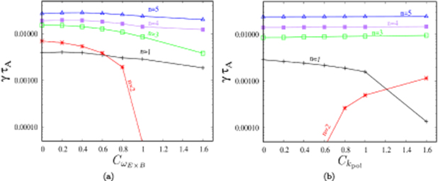
Figure 6. The effect of toroidal and poloidal rotation on the normalized growth rates. The normalized growth rates for different mode numbers are plotted as functions of scaling factors for the  and
and  profiles derived from the experiment.
Download figure:
Standard image High-resolution imageThe results presented in this section demonstrate that modeling of a saturated EHO requires an increased instability drive. As it is indicated in introduction, this is a possible outcome of large amplitude fluctuations observed in the edge that relax the edge profiles. Two equilibria, the  and
and  cases, were developed to bracket the expected range of reasonable instabilities. These cases were characterized with respect to the linear instability, and both were determined to be suitable for non-linear simulation.
3. Saturated states from linear peeling-ballooning mode instabilities
The objective of this non-linear modeling is to understand how the saturated state depends on the initial profiles. Global validation consists of comparing the profiles of the saturated steady state to the experimental profiles. This determines if the saturated perturbation can drive particle and thermal transport strong enough to relax steep density and temperature profiles towards the experimental profiles.
NIMROD simulations are performed with 22 toroidal modes. In order to ensure sufficient resolution for high-n mode numbers, the poloidal mesh is composed of 72 × 128 bi-quintic spectral elements. Spitzer resistivity enhanced by a factor of 3 is used. The enhancement of the resistivity is justified by the lack of inclusion of impurities in the NIMROD code [8]. In the experiment,  can change in a relatively wide range in this region. In particular,
  exceeds 5 in the QH-mode pedestal region of the DIII-D discharge 163 518. However, there are relatively high uncertainties in the evaluation of
  in this region. A new model for impurities that is currently being developed that will help to account the variation of the Spitzer resistivity more accurately. Other main physics parameters include the isotropic particle diffusivity of 1 m2/s, the parallel viscosity of 105
m2/s, and the isotropic viscosity of 1 m2/s on axis. The anisotropic thermal conduction model is used with the parallel ion and electron thermal conductivities of 107
m2/s and perpendicular conductivities of 1 m2/s. The isotropic viscosity and perpendicular thermal conduction are increased from 1 m2/s to 3 m2/s in the NIMROD simulation of the
in this region. A new model for impurities that is currently being developed that will help to account the variation of the Spitzer resistivity more accurately. Other main physics parameters include the isotropic particle diffusivity of 1 m2/s, the parallel viscosity of 105
m2/s, and the isotropic viscosity of 1 m2/s on axis. The anisotropic thermal conduction model is used with the parallel ion and electron thermal conductivities of 107
m2/s and perpendicular conductivities of 1 m2/s. The isotropic viscosity and perpendicular thermal conduction are increased from 1 m2/s to 3 m2/s in the NIMROD simulation of the  case.
case.
The simulations for both cases converge to saturated states with n = 1 as the dominant mode. The simulations for the equilibrium with a stronger initial instability drive ( ) saturates at significantly higher levels as compared to the
  case as shown in figure 7. The saturated kinetic and magnetic energy associated with n = 1 mode is three orders of magnitude larger for the
  case comparing to the
  case, even thought the gradient is only 70% larger. One could expect that the larger mode amplitudes for the larger gradient will result in larger relaxation. It is interesting that the n = 1 mode becomes nonlinearly dominant for both cases, given the linear stability results shown in figure 4.
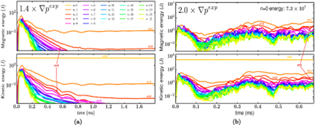
Figure 7. Magnetic and kinetic energies as functions of time for different modes numbers. The plots on the left (a) are computed for the  case. The plots on the right (b) are computed for the
  case. The simulations for the equilibrium with a stronger initial instability drive saturate at significantly higher levels as well as showing richer mode activity.
Download figure:
Standard image High-resolution imageFigure 8 shows relaxation of the flux-surface-averaged plasma profiles for both cases. The profiles are shown as functions of the normalized toroidal flux. The initial profiles (representing  )) are shown as black solid curves and final profiles are shown as red dashed curves, indicating the final 2D state (
 ). The final profiles are averaged over final 0.011 ms of the simulations. The experimental data for electron temperature and density are shown as points. The first step in validating NIMROD is the comparison of these final states with the experimental profiles (
 ) serves as our first validation metric [24].
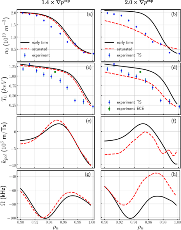
Figure 8. Flux-surface-averaged profiles of density n0 (a) and (b), temperature T0 (c) and (d),  (e) and (f) and toroidal rotation rates (g) and (h) as functions of the normalized toroidal flux for the
  (left) and
  (right) cases. Initial profiles (
 ) are shown as black curves, and final profiles (
 ) are shown as red curves. Experimental data (
 ) for the electron temperature and density is shown as points with error bars. The
  case is under-driven: the equilibrium profiles are not strong enough to drive the instabilities to relax the profiles to the experimental values. The
  case is over-driven: the instabilities relax the profiles to the beyond the experimental values.
Download figure:
Standard image High-resolution imageBoth density and temperature profiles relax the initial stiff profiles towards the profiles derived mostly from the DIII-D Thomson scattering (TS) measurements [25]. As seen for the  case, the density and temperature profiles do not completely relax to the measured profiles; thus, we characterize this equilibrium as being under-driven. In contrast, the final density profile for the
  case is found below the measured values and thus we can say that it is over-driven. Interestingly, the temperature does not seem as far off as the density. Both profiles however show significant changes near the pedestal top. These changes can be attributed to the transport model used in the simulation that includes radially flat diffusivity profiles. It should be noted that in the simulation for the
  case uses the diffusivity coefficients enhanced by factor of three compared to the simulation for the
  case. The enhanced diffusivity coefficients were necessary as a computational practicality in simulating this over-driven case—the dynamics were so violent that numerical challenges arose. From considerations of the density and temperature profiles, we hypothesize that a better equilibrium is between these two cases. This more accurate case would be easier to simulate than the over-driven case. This issue will be revisited in subsequent Sections.
The relaxation of the profiles due to the modes includes the toroidal and poloidal rotation profiles as seen in the bottom 4 subfigures of figure 8. The definition of  is given in the discussion leading to equation (2) and Ω is defined as
  . As discussed in section 2, the initial flow profile is not changed from a profile that is based on a fit to the flow inferred from CER measurements for carbon impurities. For the
  , or under-driven, case, there is modest changes over the course of the simulation. However, the
  , or over-driven, case shows significant relaxation in both the toroidal and poloidal flow profiles. The poloidal flow profile also shows the development of additional structure within the profile. We will discuss these profiles in more detail when the frequency dependence of the synthetic-diagnostic results are discussed.
Also useful in understanding the results of the local synthetic diagnostic, is examining the flux-surface-averaged density and temperature perturbations as shown in figure 9 for the  . The maximum density perturbations at the end of the simulation are shifted away from the separatrix relative to the location of the perturbations at earlier time. This change reflects a shift in the instability drive due to the profile relaxation. In contrast to these results, the plasma profiles do not change much for the case
  ; i.e. the under-driven case shows small perturbations that do not significantly change location relative to the localization of the linear perturbations. For this case, the most affected quantity is found to be the toroidal rotation rate that is relaxed by 10% in the pedestal region compared to the initial profile.

Figure 9. Flux-surface-averaged profiles of density density (a) and temperature perturbation for the  case. Profiles averaged over initial 0.15 ms are shown as black curves, and final profiles averaged over final 0.011 ms are shown as red curves. The peak of the saturated non-linear perturbations amplitude shifts inward relative to the linear perturbation amplitudes for this EHO case.
Download figure:
Standard image High-resolution imageSummarizing, the non-linear results for the  and
and  cases, one can see that both cases result in saturated states with the most dominant low-n modes that are similar to the dominant modes observed in experiment. In both cases, the n = 1 becomes the dominant mode. Examination of the relaxed profiles indicate that
  is under-driven; i.e. the drive is not strong enough to relax the profiles to the measured values; while
  is over-driven; i.e. the profiles are steepened to much and the profiles relax too much. The flow profiles for this over-driven case also relax and deviate strongly from the measured values. In order to make a final conclusion how these two cases resemble measurements a direct comparison with local diagnostics is necessary. This topic is addressed in the next section.
4. Validation of saturated states using localized synthetic diagnostic
In this section, a synthetic beam emission spectroscopy (BES) diagnostic is used to further validate the saturated states for the  and
and  cases. For DIII-D discharge 163 518, the BES experimental diagnostic [26] detects density perturbations with frequencies in the range from 0 to 80 kHz in the QH-mode pedestal region. Being integrated over this frequency range, the maximum density perturbations are found around 2.5-3% in the experiment. The measurements are localized at the outer midplane pedestal region.
As a first step, it is useful to consider the relationship of these localized measurements to the overall simulation results. Figure 10 shows contour plot of electron density for the  case. The density perturbations are mostly localized around X-points and have minimal values at the location of the 64 BES channels that are located within the white box shown in the figure. These localized measurements will naturally show smaller density perturbations than the density perturbations for the the averaged profiles shown in the previous section.

Figure 10. Contour plot of electron density for the  case. The BES system location is marked with a white box.
Download figure:
Standard image High-resolution imageNonetheless, it is useful to consider the flux-surface-averaged density perturbations shown in figure 11. For the  case, the maximum density perturbation exceeds 25% and for the
  case, the density perturbation is approximately 1%. In the flux expansion regions, the density perturbations exceed 30% for the case with a stronger instability drive and remains within several percent for the case with a weaker instability drive. The instability drive plays a critical role in establishing the perturbations levels in the saturated states. Although the flux-surface-averaged quantities will likely be higher than our localized measurements because they include the large perturbations near the X-point, it is clear from these plots and the BES measurements that
  is indeed under-driven, and
  is over-driven. What is perhaps surprising is that while the relaxed global profiles in figure 8 make it appear that
  is closer to the optimal equilibrium, the local perturbations means that
  is closer to optimum.

Figure 11. Normalized flux averaged density perturbation profiles as functions of normalized toroidal flux for the  (a) and
  (b) cases.
Download figure:
Standard image High-resolution imageThis comparison of the amplitude of NIMROD density perturbations with the experimental density perturbations is a convenient way to compare the modeling results with experimental data. However, a more direct comparison through a synthetic BES diagnostic in NIMROD can provide an immediate mechanism for the validation of modeling results. The synthetic BES diagnostic is implemented in the NIMROD framework. Using this approach, the synthetic density  is
is
where ne
is the electron density computed with the NIMROD code and  is the point spread function (PSF) [27], the same function that also used in the BES experimental analysis. Figure 12 shows the location of the BES channels in the experiment and in the simulation. The separatrix location in the equilibria used to initialized the NIMROD simulation does not exactly coincide with the separatrix location in the experimental reconstruction due to the changes in the equilibrium re-solve discussed in section 2. In order to maintain the relative location of the BES diagnostic relative to the separatrix location, the BES array is shifted several centimeters outward as shown in figure 12 for the
  case.
case.
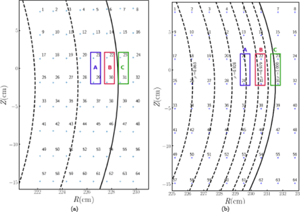
Figure 12. Location of the BES channels in experiment (a) and in simulation for the  case (b).
Download figure:
Standard image High-resolution imageIn the experiment, there are slow and fast channels that effectively separate the emission signals into the averaged density and perturbation density. The slow BES channels in the experiment as well as plasma profiles in the NIMROD simulations are not completely in a perfect steady state. The experimental slow BES signals can slowly vary in time. These variations are typically fluctuate in time and they might introduce artificial frequencies to the BES spectral analysis. In order to exclude these frequencies, the BES experimental analysis is performed over multiple overlapping time windows [28]. In the NIMROD simulations, there are no such variations in the averaged profiles. However, the transport model contributes to profile evolution as it is indicated in section 3. The synthetic BES channels include contributions both from MHD instability dynamics,  and from the transport model,
  :
:

The time-averaged signals  is approximately equal to
  , because
  and
and  are expected to be zeros when they are being averaged over sufficiently large time-frames. The
  value corresponds to the slow BES channel in experiment, and
  corresponds to the fast channel. The transport model with constant diffusivity coefficients typically yields local changes that either increase or decrease in time. Effectively, the
  introduces an artificial frequency to the BES analysis at the FFT numerical resolution frequency. In order to remove this artifact from the synthetic BES analysis, time-averaging is replaced with the averaging over toroidal angle. In this analysis, the synthetic density is averaged over 50 random toroidal angles for each individual time. Using this approach, the fast channel does not includes the
  term and becomes equal to
  .
.
The experimental BES analysis often includes the computation of the cross-correlation which is a measure of similarity of two time series. It is defined as

where I is the fast BES signal,  is the BES signal at the BES reference channel, and τ is the time delay. The summation is performed over multiple fast BES measurement times tn
. The time window for the cross-correlation analysis in experiment is typically include 1000 measurements at 1 MHz frequency. Due to the large computational cost of the simulation, the integration time window was limited to the last 0.55 ms at the end of simulations shown in figure 7 for the
is the BES signal at the BES reference channel, and τ is the time delay. The summation is performed over multiple fast BES measurement times tn
. The time window for the cross-correlation analysis in experiment is typically include 1000 measurements at 1 MHz frequency. Due to the large computational cost of the simulation, the integration time window was limited to the last 0.55 ms at the end of simulations shown in figure 7 for the  case and the last 0.20 ms for the
  case, which corresponds to 550 and 200 individual time slices correspondingly. The density perturbations that are proportional to the fast BES signals are used to compute the cross-correlation function
  at the BES channel locations. Figure 13 shows the cross-correlation of the BES synthetic signal for the
  case. The EHO is represented by a large structure localized in the pedestal region that slowly rotates in the ion diamagnetic drift direction.
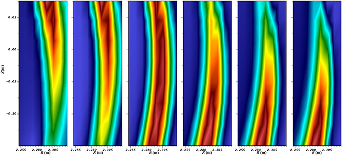
Figure 13. Cross-correlation of the synthetic BES signal at consequent 7 µ
sec time delays for the  case. The BES channel 14 in figure 12 is selected as the reference channel.
Download figure:
Standard image High-resolution imageThe cross-power spectral density analysis provides important information on the perturbation spectra [28]. The normalized synthetic density perturbations for channels 21/29 (channels A in figure 12), 22/30 (channels B in figure 12), and channels 23/31 (channels C in figure 12) are used to compute cross-power spectral density. The experimental and synthetic cross-power spectral densities are compared in figure 14(a)–(c). A narrower spectrum of perturbations is observed in the simulation results. This is particularly true for the  case. For the
  case, several additional frequencies are presented in the spectrum shown in figures 14(a–c). However, they do not extend to 80 kHz as in the experimental spectrum. The amplitude of cross-power spectral density for this case is also significantly lower comparing to the experimental cross-power spectral density and synthetic cross-power spectral density for the
  case. Note the scaling factors of 2 and 0.004 that is used to for the cases
  and
and  to plot the synthetic spectral density on the same scale as the experimental spectral density. The differences in the spectral density amplitudes approximately agree with the differences in the normalized density perturbations shown in figure 11 and agree with the previous observation that the case
  is under-driven and the case
  is over-driven.
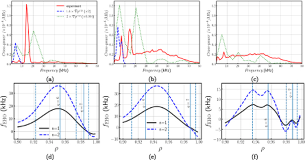
Figure 14. Cross-power spectral densities computed for normalized density perturbations and rotation frequencies for the n = 1 and n = 2 modes. The cross-power spectral densities are shown as functions of frequency for channels 21/29 (a), 22/30 (b), and 23/31 (c) as shown in figure 12. The BES experiment data are shown as solid curves and the synthetic BES simulation data are shown as dashed curves for the  case and as dotted curves for the
  case. The rotation frequencies are computed using equation (6) for the experimental profiles (d),
  (e), and
  (f) cases and are shown as functions of normalized toroidal flux. The location of resonant surfaces are shown in solid and dashed vertical lines.
Download figure:
Standard image High-resolution image
The spectral properties of synthetic cross-power spectral densities are notably different from the experimental observation. In the experiment, EHO is represented by a large coherent structure that slowly rotates at a fixed rate. It is expected that there is one dominant mode that determines this rotation. There is one peak in experimental cross-power spectral density for the BES channels that are localized in the pedestal region. In particular, one peak in experimental cross-power spectral density appears in figures 14(a) and (b) at approximately the same frequency of 15 kHz. The second peak at 6.8 kHz appears in figure 14(b). It likely corresponds to a sub-dominant mode. There is a similar transition from single to a double-peak structure for the  case. However, there are two peaks that appear for both sets of BES channels in the pedestal region for the
  case. Larger cross-power spectral densities are associated with the first peak for both
  and
and  cases. It is specially true for the BES channels that are located next to separtix. In the experiment, the second peak carries more spectral energy density comparing to the first peak. The frequencies of peaks for the case
  are different from the frequencies of peaks in experiments. These frequencies are at approximately 5.2 kHz and 20.6 kHz. The BES channels for the
  case are kept at the locations of the BES channels in experiment. Because of the separatrix shift during the equilibrium reconstruction, the last BES channel at the midplane is 0.5 cm inside from the area marked with letter B in figure 12.
The EHO rotation in the poloidal direction that is responsible for the second peak in the cross-power spectra for the  case is larger than the frequencies of both peaks in the experimental spectra. The EHO rotation frequency can be estimated as the local rotation rate:

where n is the mode number, q is the safety factor,  , and V(ψ) is the plasma volume contained within the surface ψ. Figure 14(d)–(f) shows the rotation frequency as a function of normalized toroidal flux for the experiment,
  and
and  cases respectively. This estimate utilizes some flux surface average quantities from figure 8. The estimates of EHO rotation frequency in figures 14(d)–(f) show that the frequency depends on the mode localization.
The estimated rotation frequencies in figure 14(d) can explain the experimental peaks that are shown as red curves in figures 14(a) and (b). The large peak at approximately 15 kHz in figure 14(a) is close to the rotation frequency of n = 1 mode at ρ = 0.954 (and q = 6) and n = 2 mode at ρ = 0.974 (and = 6.5) in figure 14(d). These two modes are likely to define the rotation of EHO in the experiment. The n = 2 rotation frequency is also in agreement with the spectrogram n = 2 frequency shown figure 1. As a dominant mode, n = 2 extends to several channels and is present in figure 14(b) for the BES channels 22/30. The n = 1 mode at ρ = 0.984 (and q = 7) is the most likely candidate to explain the first peak in this figure.
Similar to the experiment, both  and
and  cases show the transition from single to a double peak structures in the cross-power spectral densities. However, the first peak in the
  case is found lower than the experimental frequencies and the second peak in the
  case is found larger than the experimental frequencies. The second peak in the
  case in figure 14(b) matches the first peak in the spectral density analysis for the experiment. It is likely to be associated with the n = 2 mode at ρ = 0.995 (and q = 7.5). It has approximately the same frequency as in the rotation frequency estimate at this location in figure 14(e). The n = 1 mode at ρ = 0.988 (and q = 7) is consistent with the first peak in figure 14(b). Note that the density perturbations in this case are very localized close to the separatrix as shown in figure 11(a).
The peaks in the cross-power spectral densities for the  case are expected to be at different frequencies than the experimental peaks. Figure 8 shows that the density and temperature profiles evolve toward the experimental density profiles. The maximum density perturbation location shifts from ρ = 0.97 in the beginning of the simulation to ρ = 0.96 at the simulation end (see figure 9). However, the simulation is initialized with the experimental toroidal and poloidal rotation profiles and these profiles evolve at the simulation end. As result, there is a misalignment between the maximum density perturbation location, which evolved towards maximum density gradient location observed in the experiment and relaxed rotation profiles. Both n = 1 mode at ρ = 0.956 (q = 6) and n = 2 mode at ρ = 0.98 (q = 6.5) and at ρ = 0.993 (q = 7.5) can contribute to the first frequencies peak in figures 14(a) and (b). As it is shown in figure 14(f), both modes are expected to rotate at low frequencies that are within the FFT resolution frequency of the first peak in figures 14(a) and (b). We hypothesize that the second peak in figure 14(b) for this strongly over-driven case can be explained by MHD turbulence bursts that are observed in the local analysis of density perturbations for n = 1 and n = 2 modes at the location of the BES measurements that is shown in figure 15(a). The results of FFT analysis figure 15(b) of these perturbations shows peaks at low and 20 kHz frequencies.

Figure 15. (a) Density perturbations for the n = 1 and n = 2 modes at a diagnostic localized between the BES channels 22 and 33 (channels B) in figure 12 as functions of time. (b) FFT of the density perturbation at the local probe.
Download figure:
Standard image High-resolution image
For both  and
and  cases, the cross-power spectral density is larger for the first peak. The EHO rotation is expected to be determined by the n = 1 mode that remains mostly responsible for the first peaks in figure 14(b). The dominant role of n = 1 mode agrees with the kinetic and magnetic energies associated with different toroidal modes in figure 7. It also highlights the difference with the experiment, where the EHO rotation is likely determined by the n = 2 mode.
5. Discussion and conclusions
In this research, the EHOs in the DIII-D discharge 163 518 are simulated using the NIMROD code. The equilibrium is based on the EFIT reconstruction at time 2350 ms, when saturated EHO is observed, is found stable in the ELITE and NIMROD codes. This result indicates the fact that saturated perturbations drive the particle and thermal transport to maintain steady-state pedestal profiles. Two unstable kinetic equilibria are generated using EFIT by adjusting the QH-mode pedestal width. The weakly-driven equilibrium has the maximum pressure gradient in the QH-mode pedestal approximately 1.4 times larger than the maximum pressure gradient in the experiment (the  case). The strongly-driven equilibrium has the maximum pressure gradient two times larger than the pressure gradient in the experiment (the
  case).
The effects of toroidal and poloidal rotation are investigated by scaling the experimental rotation profiles in the linear NIMROD simulations. It is found that the toroidal rotation stabilizes all lower n modes considered in this scan and poloidal rotation can stabilize or destabilize these modes. However, even with significantly increased poloidal rotation, the most unstable mode remains n = 5, the largest toroidal mode number considered. The linear analysis can not explain the mode spectrum observed in the DIII-D discharge 163 518 with dominant low-n modes.
Our method of enhancing the instability drive likely does not take the correct trajectory in exploring of the ( , ∇p) peeling-ballooning stability space. As shown in figure 3, we choose to scale both the current and pressure drives roughly equally. Although this figure is only a schematic, more detailed calculations not presented here show that increasing the bootstrap current more than just that given by the pressure gradient steepening gives unstable equilibria with less change to the equilibrium. In terms of the schematic, this represents making our lines from
  to
u0
more vertical. This can be done while staying within the uncertainties of both calculating the bootstrap current and experimental observations.
to
u0
more vertical. This can be done while staying within the uncertainties of both calculating the bootstrap current and experimental observations.
Remarkably however, given these caveats and uncertainties, in the non-linear NIMROD simulations perturbations for both equilibria saturated to states with n = 1 as the dominant mode number. Although our sample size is small, this suggests that the accessibility of the QH-mode, and similar regimes, is larger than that suggested purely by linear analysis. Specifically, one would not guess a priori that an equilibrium with flow that has the n = 5 as the most unstable mode would yield a non-linear state with n = 1 being dominant. A caveat to these simulations is that our initialization favored the lower n modes. This suggests that experimentally a low-n perturbation could be used to kick the plasma into the desired non-linear state.
The kinetic and magnetic energies associated for the n = 1 mode in these saturated states is found differ by three orders of magnitude. For the case with a stronger instability drive, the profiles relaxes towards the experimental profiles with larger changes observed in the density profile. For the case with a weaker instability drive, the changes in the profiles are significantly smaller comparing to the case with a stronger drive. The transport in the  case is also not strong enough to relax the profiles to the experimental profiles.
The global flux-averaged profiles make it look like the  case is closer to the experiment, but the
  case looks closer when considering perturbation size and the BES diagnostic. This shows the value of local validation. From the comparison of the density perturbation levels in the QH-mode pedestal with the BES experimental data, it is found that the perturbation level is significantly larger than in the experiment for the
  case and smaller for the
  case. The EHO saturation level is sensitive to the equilibrium plasma profiles. In these simulations, change in the pedestal width by 20% yields a difference in the saturated density perturbations by a factor more than 20.
The validation of NIMROD results is improved by implementing the BES synthetic diagnostic in the NIMROD framework. In the NIMROD synthetic BES analysis, the BES channels are shifted in order to account for a shift in separatrix in the equilibria with the modified pedestal profiles. The use of the BES synthetic diagnostic is demonstrated by computing the cross-correlation for the density perturbations at the locations of the experimental BES channels and by computing the cross-power spectral densities and comparing them with the experimental cross-power spectral densities. Based on a frequency analysis using equation (6), it is shown that n = 1 and n = 2 are the main contributors to the experimental cross-power spectral density at the BES channels located at ρ = 0.96 and ρ = 0.98. There is a transition from a single peak structure in the cross-power spectral density at ρ = 0.96 to a double peak structure at ρ = 0.98. Similar trend in the cross-power spectral densities is reported for the  and
and  cases. The n = 1 and n = 2 modes explain both frequency peaks for the
  case and the first peak for the
  case. The
  case is found to be strongly over-driven with a periodic MHD turbulence bursts that contribute to the second peak in the cross-power spectral density at approximately 20 kHz.
While the synthetic BES diagnostic shows that the simulations here do not exactly reproduce the fluctuations observed in the experiments, they represent substantial progress on moving towards simulations that do. In particular, future simulations where instability drive enhancement is needed will use larger current enhancement with more modest changes to the pressure profile. Also it is clear that the flows largely determine the fluctuation rates and large fluctuation-induced torques are present in the simulation that significantly modify the rotation profiles. However, as other large edge torques, such as those from ion orbit loss and neutrals, are not properly accounted for, future simulations will constrain the rotation profile to more closely match experiment. After validation of the fluctuation dynamics through comparisons with local diagnostics such as BES, the next step is integration with pedestal transport physics outside MHD to move towards more predictive modeling of QH dynamics.
Acknowledgments
The primary author wishes to thank Dr Tariq Rafiq for reviewing the paper and discussions, and Dr Eric Howell for discussions about the interpretation of the EHO rotation frequencies BES analysis.
This material is based on work supported by the U.S. Department of Energy Office of Science and the SciDAC Center for Extended MHD Modeling under contract numbers DE-SC0019070, DE-SC0018311, DE-SC0020251 (Tech-X collaborators), and DE-FC02-04ER54698 (General Atomics collaborators). This research used resources of the National Energy Research Scientific Computing Center, a DOE Office of Science User Facility supported by the Office of Science of the U.S. Department of Energy under contract No. DE-AC02-05CH11231.
DISCLAIMER: This report was prepared as an account of work sponsored by an agency of the United States Government. Neither the United States Government nor any agency thereof, nor any of their employees, makes any warranty, express or implied, or assumes any legal liability or responsibility for the accuracy, completeness, or usefulness of any information, apparatus, product, or process disclosed, or represents that its use would not infringe privately owned rights. Reference herein to any specific commercial product, process, or service by trade name, trademark, manufacturer, or otherwise, does not necessarily constitute or imply its endorsement, recommendation, or favoring by the United States Government or any agency thereof. The views and opinions of authors expressed herein do not necessarily state or reflect those of the United States Government or any agency thereof.