

Abstract
Objective. Revealing the relationship between simultaneous scalp electroencephalography (EEG) and intracranial electroencephalography (iEEG) is of great importance for both neuroscientific research and translational applications. However, whether prominent iEEG features in the high-gamma band can be reflected by scalp EEG is largely unknown. To address this, we investigated the phase-amplitude coupling (PAC) phenomenon between the low-frequency band of scalp EEG and the high-gamma band of iEEG. Approach. We analyzed a simultaneous iEEG and scalp EEG dataset acquired under a verbal working memory paradigm from nine epilepsy subjects. The PAC values between pairs of scalp EEG channel and identified iEEG channel were explored. After identifying the frequency combinations and electrode locations that generated the most significant PAC values, we compared the PAC values of different task periods (encoding, maintenance, and retrieval) and memory loads. Main results. We demonstrated that the amplitude of high-gamma activities in the entorhinal cortex, hippocampus, and amygdala was correlated to the delta or theta phase at scalp locations such as Cz and Pz. In particular, the frequency bin that generated the maximum PAC value centered at 3.16–3.84 Hz for the phase and 50–85 Hz for the amplitude. Moreover, our results showed that PAC values for the retrieval period were significantly higher than those of the encoding and maintenance periods, and the PAC was also influenced by the memory load. Significance. This is the first human simultaneous iEEG and scalp EEG study demonstrating that the amplitude of iEEG high-gamma components is associated with the phase of low-frequency components in scalp EEG. These findings enhance our understanding of multiscale neural interactions during working memory, and meanwhile, provide a new perspective to estimate intracranial high-frequency features with non-invasive neural recordings.
Export citation and abstract BibTeX RIS
Abbreviations
| EEG | electroencephalography |
| iEEG | intracranial electroencephalography |
| PAC | phase-amplitude coupling |
| MNI | Montreal Neurological Institute |
| GLM | general linear model |
| ECL | left entorhinal cortex |
| ECR | right entorhinal cortex |
| AHL | left hippocampal head |
| AHR | right hippocampal head |
| AL | left amygdala |
| AR | right amygdala |
| PHL | left hippocampal body |
| PHR | right hippocampal body |
| fMRI | functional magnetic resonance imaging |
1. Introduction
As a non-invasive measure modality, scalp electroencephalography (EEG) recording has been widely used as a diagnostic tool for epilepsy and other neurological diseases [1], and also brain-triggered therapies for stroke and severely disabled patients [2, 3] due to its excellent temporal resolution and the whole coverage. However, scalp EEG is limited by its low spatial resolution and signal quality [4]. In contrast, intracranial electroencephalography (iEEG) can capture activities at both the cortex and deeper brain structures with millimeter-level spatial resolution and a higher signal-to-noise ratio [5]. Meanwhile, the operation of iEEG is always limited in intractable epilepsy patients because of its risk of craniotomy. Therefore, revealing the relationship between scalp EEG and iEEG is crucial for estimating intracranial features as possible using more accessible scalp measurements [6]. To this end, simultaneous recordings of scalp EEG and iEEG are essential for investigating the relationship between the same neural representations reflected by two types of signals [7].
In simultaneous EEG and iEEG studies, correlation analysis is commonly used to evaluate the relationship between the superficial and intracranial signals. Based on this method, it was reported that time series of scalp EEG components could be highly correlated with iEEG signals of a local brain region [8]. Besides, Seeber et al have also found a significant correlation between the envelope of iEEG and the envelope of source signals reconstructed by high-density scalp EEG [9], and the highest correlation was obtained by source signals in close proximity to the actual depth contacts. Based on multi-channel signals of macaques, a study adopted canonical correlation analysis to evaluate how much information was shared between the subsets of the EEG components and iEEG signals [10], where different source reconstruction algorithms for EEG showed differentiated performances. In addition to the above studies using rest-state data, a visual stimulation paradigm revealed that concordant patterns between scalp EEG and iEEG were found below the 40 Hz level in the average time-frequency domain [7]. In general, most previous simultaneous EEG and iEEG studies focused on the low-frequency components of iEEG (below 60 Hz), or only investigated the relationship between scalp EEG and low-frequency iEEG [11]. However, few studies identified the correlation between scalp EEG and high-frequency iEEG components above 60 Hz. In a macaques' action observation and execution task, Bimbi et al found that the increase of high-gamma (63–100 Hz) power in the intracranial recordings was correlated to beta and partial alpha desynchronization of scalp EEG [12]. So far, similar studies involving high-gamma band is rarely reported.
Notably, it is crucial to study the high-gamma activities of iEEG recordings since the component in this frequency band may reflect the population-level neuronal firing [5, 13], and hence plays a significant role in clinical applications and neural mechanism research. More specifically, high-gamma activities have been suggested to correlate with seizure onset zones [14], and this frequency band can also serve as biomarkers to distinguish interictal and ictal states [15]. Additionally, high-gamma activities can work as reliable indexes for functional areas mapping [16, 17] and provide informative features for discriminating different movements and mood states [18, 19]. It's generally believed that body tissues such as the skull and scalp behave as a low-pass filter for brain signals, making the high-frequency components of cortical neural signals (above 40 Hz) hard to be reflected in scalp EEG [20]. Nevertheless, it is still possible to predict certain features of the high-frequency activity in iEEG recordings using scalp EEG signals, based on the reported power coupling phenomenon between intracranial high-gamma band and the beta band on the scalp [12].
In addition to the power coupling, the phase-amplitude coupling (PAC) might also provide a promising solution to infer intracranial high-frequency features via scalp recordings. In brief, PAC denotes that the instantaneous amplitude of a higher frequency band within a signal is modulated by (or otherwise linked to) the instantaneous phase of a lower-frequency band of the same (or a different) signal [21]. A number of studies have suggested that PAC can exist in various frequency combinations, such as theta (4–8 Hz) and high-gamma (80–150 Hz) coupling in iEEG recordings [22], delta (0.5–4 Hz) and low-gamma (30–50 Hz) coupling in scalp recordings [23]. Interestingly, significant PAC can even be observed between the delta/theta phase of iEEG and beta/low-gamma amplitude of scalp EEG, and also between the delta phase of scalp EEG and theta/alpha amplitude of iEEG [24]. However, till now, it remains largely unknown whether the amplitude of iEEG high-gamma components is associated with the phase of low-frequency components in scalp EEG.
To address this question, this study conducts a comprehensive PAC analysis using a synchronous iEEG and EEG recording dataset acquired under the verbal working memory task [25]. The results suggest that the PAC phenomenon can be detected under the working memory task, and the degree of coupling presents significant differences across different task periods and memory loads. These findings improve our understanding of intracranial-scalp neural information transmission during working memory, and meanwhile, provide a new perspective to estimate intracranial high-gamma features by non-invasive recordings.
2. Materials and methods
2.1. Subjects
The patient data we studied here were from a recent public dataset of simultaneous iEEG and scalp EEG [25]. In detail, nine right-handed subjects participated in the study. The participants were intractable epilepsy patients undergoing presurgical assessment, where depth electrodes were implanted for the iEEG recording, and scalp EEG signals were recorded simultaneously. The implantation configurations were determined strictly for clinical demands. All subjects signed informed consent before the experiment, approved by the institutional ethics review board (Kantonale Ethikkommission Zürich, PB-2016-02055) [25, 26]. More details about the subjects that participated in this study can be seen in table 1.
Table 1. Clinical profile of all subjects. Source: adapted from [25].
| Subject | Age | Gender | Pathology | Seizure onset zone contacts |
|---|---|---|---|---|
| Sub1 | 24 | F | Xanthoastrocytoma WHO II | AHR, LR |
| Sub2 | 39 | M | Gliosis | AHR, PHR |
| Sub3 | 18 | F | Hippocampal sclerosis | AHL, PHL |
| Sub4 | 28 | M | Brain contusion | AHL, AHR, PHL, PHR |
| Sub5 | 20 | F | Focal cortical dysplasia | DRR |
| Sub6 | 31 | M | Hippocampal sclerosis | AHL, PHL, ECL, AL |
| Sub7 | 47 | M | Hippocampal sclerosis | AHR, PHR |
| Sub8 | 56 | F | Hippocampal sclerosis | ECR |
| Sub9 | 19 | F | Hippocampal sclerosis | ECR AR |
Abbreviations denote the brain regions: AH for hippocampal head; PH for hippocampal body; A for amygdala; EC for entorhinal cortex; L for left; R for right; LR for lesion; DRR for dysplasia.
2.2. Data recording and electrode localization
The iEEG data were recorded with the Neuralynx ATLAS recording system (Neuralynx, Bozeman, MT, USA) against a common intracranial reference. Scalp EEG data were recorded with the NicOne system against the averaged mastoid references. In the released dataset, the sampling rate of iEEG and scalp EEG are 2000 and 200 Hz, respectively. Each depth electrode shaft contains eight contacts. The dataset also provides the normalized contact coordinates in the standard Montreal Neurological Institute (MNI) space and corresponding anatomical labels based on the Brainnetome Atlas [27]. The number of intracranial contacts in each brain region is shown in table 2. The scalp electrodes were placed according to the international 10–20 system. Each subject had 6–17 scalp electrodes and two mastoid electrodes. Scalp electrodes' locations and the corresponding number of subjects that had the electrode were shown in figure 1.
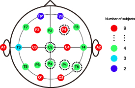
Figure 1. Locations and numbers of all available scalp electrodes. For each electrode, the number of subjects that had the electrode is marked with different colors.
Download figure:
Standard image High-resolution imageTable 2. Number of intracranial contacts.
| Subject | AHL | AHR | AL | AR | ECL | ECR | PHL | PHR | LR | DRR |
|---|---|---|---|---|---|---|---|---|---|---|
| Sub1 | 8 | 0 | 8 | 0 | 8 | 0 | 8 | 8 | 8 | 0 |
| Sub2 | 8 | 8 | 8 | 8 | 8 | 8 | 8 | 8 | 0 | 0 |
| Sub3 | 8 | 8 | 8 | 0 | 8 | 8 | 16 | 8 | 0 | 0 |
| Sub4 | 8 | 8 | 8 | 8 | 8 | 8 | 8 | 8 | 0 | 0 |
| Sub5 | 8 | 0 | 8 | 0 | 8 | 8 | 8 | 16 | 0 | 8 |
| Sub6 | 8 | 8 | 8 | 8 | 8 | 8 | 8 | 8 | 0 | 0 |
| Sub7 | 8 | 8 | 8 | 8 | 8 | 8 | 8 | 8 | 0 | 0 |
| Sub8 | 7 | 8 | 8 | 8 | 8 | 8 | 8 | 9 | 0 | 0 |
| Sub9 | 8 | 8 | 8 | 8 | 8 | 8 | 8 | 8 | 0 | 0 |
Abbreviations for brain regions are the same as the ones in table 1.
2.3. Experimental paradigm
A verbal working memory task containing the encoding, maintenance, and retrieval periods was implemented for each subject (see figure 2 for the experimental paradigm in detail). During the experiment, each trial had an 8 s length and began with a fixation period lasting 1 s. Then the stimulus set was presented, which consisted of eight consonants at the center of the screen. For one trial, the middle 4, 6, or 8 letters of the stimulus were randomly used as the memory items, determining the set size for the trial (4, 6, or 8 letters, respectively). Especially, the outer positions for the set size 4 and 6 were the letter 'X', which was never a memory item. Following this 2 s encoding period, a 3 s maintenance period started without letters presentation. After the maintenance, a probe letter appeared at the start of the retrieval period, and the subjects were asked to judge whether the probe letter was contained in the stimulus or not as rapidly as possible by pressing one of two buttons, indicating match or mismatch with the subjects' memory respectively. After the button press, the probe letter disappeared, and acoustic feedback was presented to prompt the correctness of the subjects' response. The duration of this retrieval period was 2 s. Experimental data from 50 trials were collected in one session, and each subject had 2–7 sessions in the dataset.
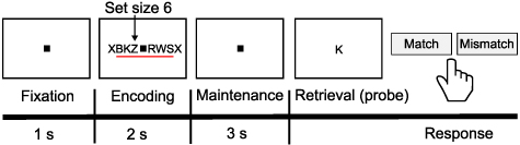
Figure 2. Experimental paradigm. A trial with a set size 6 was illustrated as an example. Figure adapted from [25].
Download figure:
Standard image High-resolution image2.4. Pre-processing and channel selection
A channel selection step was first implemented to identify the iEEG channels producing the most significant task-related responses. In the first step of channel selection, for each subject, the channels whose line noise power at 50 Hz was larger than a significance level were removed from further analysis. The significance level was defined as median line noise power across all channels plus ten times their median absolute deviation [28]. Then we performed common average reference [29, 30] in single brain regions. In brief, each channel of iEEG signal was referenced to the average of all channels with the same anatomical label. After re-referencing, we computed the power in the high-gamma (60–140 Hz) band. In detail, the signals were first band-pass filtered using a 6th order Butterworth filter. And then, we extracted high-gamma power by computing the squared absolute value of the filtered signals after Hilbert transform. For each trial, we defined the fixation period as the baseline, and normalized the power trace of the whole trial using Z-scored transformation against the baseline.
In the second step of channel selection, permutation tests were used to check whether the channel had significant responses or not [28, 31]. In detail, a single trial was divided into multiple overlapping windows with a window length of 1 s and a step length of 200 ms. For each channel, the median powers of any two adjacent windows were compared, which was implemented as follows (figure 3). First, we aligned the median value of power in the front window across all trials as x, and aligned the median in the back window across all trials as y, then concatenated x and y as z. Second, we correlated z with the corresponding front/back labels (−1/1) to obtain the Spearman r-value. Then we randomly shuffled the front/back labels and calculated the r-value between z and randomized labels. Such randomization step was repeated 1000 times, and thus, generating a Gaussian distribution with 1000 surrogate r-values. Following that, the p-value was computed, which was the percentage of the original r-value (r
 ) belonging to the Gaussian distribution. Based on this permutation test, p-values of all pairs of adjacent windows within each channel were calculated. A smaller p-value indicated a larger difference between the median values of the two adjacent windows. The channel was considered active as long as it contained p-values below the significance level (p
 0.05 after Bonferroni correction). Finally, for each channel, we extracted its minimum p-value (p
 ) across all pairs of adjacent windows. Only ten channels with the smallest p
 were kept and used in the following analysis.

Figure 3. Framework of the permutation test for iEEG channel selection. The p-value was equal to 2f( r
r

 ), where f(
 r
r

 ) was the function value corresponding to
  r
r

 .
.
Download figure:
Standard image High-resolution imageFor scalp EEG recordings, the signals were re-referenced to the averaged mastoid channels, and all EEG channels were kept in the subsequent analysis because of the relatively small number of scalp electrodes.
2.5. Analysis of PAC
The PAC values between all pairs of scalp EEG channel and the identified iEEG channel were explored using the PACTools (https://github.com/sccn/PACTools), which is an EEGLAB plug-in on Matlab platform [21, 32, 33]. Here we adopted the default approach of the toolbox, the general linear model (GLM) [34, 35], to compute PAC values in the processed data. GLM approach was initially proposed to enhance the applicability of PAC computation at 1/4 or 3/4 of the low-frequency cycle [34]. In brief, the PAC is estimated from the portion of variance explained by the linear model, and the high-frequency amplitude At is modeled by a multiple regression:

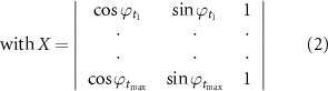
where β are regression coefficients, e is additive Gaussian noise. The matrix X is comprised of three columns: the first two columns are the sine and cosine of the low-frequency phase series (ϕt ) respectively, and the third is a constant vector of ones [21, 34].
Using PACTools, the calculations were first implemented based on all trials of the subject to find effective channel pairs and frequency combinations. In detail, the PAC phenomenon was searched in wide frequency ranges, where the range of frequency for phase was 2–12 Hz divided into 15 bins, and the range of frequency for amplitude was 30–140 Hz divided into 10 bins. We set a time point every 100 ms on the time series of each 8 s trial, and thus the PAC matrix (frequencies for phase × frequencies for amplitude) was computed at these time points using each pair of channel combination. For each channel pair, the average PAC matrix across time points was regarded as its PAC measurement here.
After the PAC searching using all pairs of channel combination, we concentrated on the maximum PAC value (PAC ) extracted from the PAC matrix of each channel pair. For each subject, we identified the top 10% of the channels pairs producing the highest PAC
 value across all available pairs and termed these identified pairs as the effective channel pairs. As a consequence, there were 119 effective channel pairs in total, and effective PAC
 values in the following analysis were all from these channel pairs. Then, we identified the frequency combination corresponding to the PAC
 and the channel locations contributing to these effective channel pairs.
2.6. Validation of PAC values
To validate the resulting PAC values, we added two control groups, where the actual PAC values were compared with surrogate PAC values resulting from other low-frequency baselines. Two types of low-frequency baselines were considered. For the first type of baseline, we matched each subject with another subject that had equal experimental sessions. In this case, we implemented the same PAC calculation using all trials within the subject but replaced the scalp EEG with another subject's scalp EEG (exchanged EEG). And then, we again identified the top 10% of the channel pairs producing the highest PAC value (as section 2.5), and thus PAC matrixes and PAC
 values from 119 cross-subject channel pairs could be obtained. The second type of low-frequency baseline was defined as the sum of fixed sinusoids with different frequencies, which were set as 2–12 Hz divided into 15 bins (same as the frequency for phase in section 2.5). In this case, the scalp EEG of each trial was replaced by the same combination of fixed sinusoids, and we calculated the PAC between the combination of fixed sinusoids and all selected iEEG channels (90 in total), generating 90 surrogate PAC matrixes and PAC
 values. Subsequently, PAC matrixes and PAC
 values calculated using the actual EEG, exchanged EEG, and combination of sinusoids were compared (Kruskal–Wallis test).
2.7. Comparison among task periods and memory loads
We further compared the PAC values of different periods (encoding, maintenance, and retrieval) during the task. Briefly, for each effective channel pair, PAC matrixes belonging to the encoding, maintenance, and retrieval period were averaged across time points, respectively. Then PAC was extracted from the average PAC matrix for each of these periods, generating one PAC representative value for each period respectively. Using data from all effective channel pairs of all subjects, we applied a Kruskal–Wallis test to evaluate the differences among PAC
 of the three periods. Additionally, to investigate the PAC difference among different memory loads (i.e. set size = 4, 6, or 8), trials were grouped according to their set size, and then we re-computed the corresponding PAC matrix of effective channel pairs for each type of set size separately. Subsequently, the PAC
 under these three set size groups were compared (Kruskal–Wallis test).
3. Results
3.1. High-gamma responses of active iEEG channels
Figure 4 shows the time-frequency map of a representative active iEEG channel for each subject (computed and plotted with EEGLAB toolbox). Results suggested that the response patterns across brain regions and subjects were quite different. In the examples, sub-bands of high-gamma also responded distinctly. Despite the individual difference, all subjects had significant high-gamma responses to the working memory task.

Figure 4. Examples of time-frequency power plot for each subject. Time '0' indicates the onset of the probe letter. Each sub-figure shows the result of a typical iEEG channel with significant responses, marked with the corresponding subject and the anatomical label. Abbreviations for anatomical labels are the same as the ones in table 1. Event-related spectrum perturbation (ERSP) value is used for the visualization.
Download figure:
Standard image High-resolution imageFurther, we calculated the median time trace of high-gamma power (60–140 Hz) across trials under three different types of set size for these channels separately (figure 5, same channels as shown in figure 4). Results showed that in certain periods, the high-gamma response strength presented differentiation among the three levels of memory load. For example, in the encoding period (from −5 to −3 s) of subject 6 and the retrieval period (after 0 s) of subject 8, a larger set size elicited a higher power increase. Besides, set size 6 and 8 also resulted in higher power than set size 4 in the maintenance period (from −3 to 0 s) of subject 5.

Figure 5. Examples of high-gamma power time traces. The presented time traces indicate the median value across trials, convoluted with a 500 ms Gaussian window for visualization purposes. Time '0' denotes the onset of the probe letter. These representative active channels were the same as the ones in figure 4.
Download figure:
Standard image High-resolution image3.2. PAC between low-frequency and high-gamma bands
Significant PAC could be generated by the above iEEG channels. Figure 6(A) shows a typical PAC relation between the delta band of scalp EEG and high-gamma band of iEEG, where the amplitude envelope of high-gamma activity increased significantly after the peak of delta oscillation (zero phase) and then decreased in each cycle of delta oscillation. Moreover, our results showed that PAC phenomenon widely existed in each subject. As could be seen from the example for each subject (figure 6(B)), for most channel pairs, the most significant PAC values tended to locate at the range of around 50–80 Hz for iEEG amplitude and 2–4 Hz for the scalp EEG.
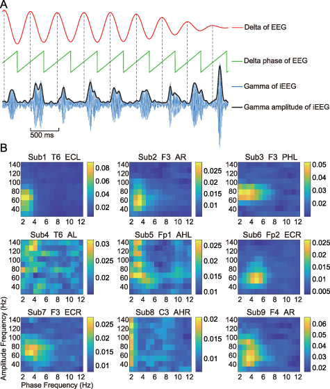
Figure 6. Examples of PAC phenomenon. (A) shows a typical PAC relation between the delta band of scalp EEG and high-gamma band of iEEG signal. This example is extracted from a trial of subject 1. (B) shows an example of PAC matrix for each subject. In all sub-figures, the horizontal ordinate indicates the frequency for scalp EEG phase, and the vertical ordinate indicates the frequency for iEEG amplitude. Each sub-figure is marked with the scalp EEG channel and iEEG channel that generated the PAC matrix. Abbreviations for iEEG channels are the same as the ones above.
Download figure:
Standard image High-resolution imageUsing the PAC value of the identified effective channel pairs from all subjects, we conducted a group analysis with respect to the center of frequency combinations and spatial locations of the PAC. Results showed that the PAC
 located most frequently in the band of 2–4 Hz for scalp EEG phase (figure 7(A)), and 39% of PAC
 values (n = 46, 119 in total) were located in the frequency bin of 3.16–3.84 Hz (figure 7(A)). For iEEG amplitude, 70 PAC
 values were found located in the 50–85 Hz band, accounting for 59% of the total (figure 7(B)). When averaging the PAC matrix across effective channel pairs, the results showed that the maximum was located at around 3 Hz for phase and 80 Hz for amplitude (figure 7(C)).
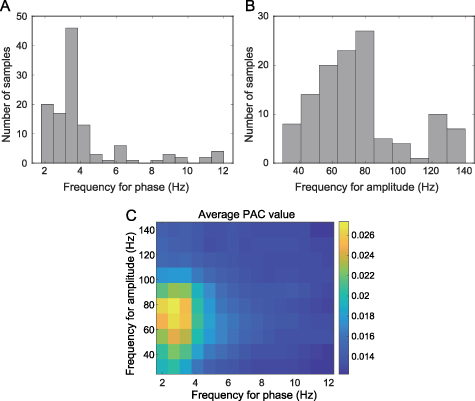
Figure 7. Histogram for frequency bands generating the PAC . (A) shows the histogram of frequency for scalp EEG phase. (B) shows the histogram of frequency for iEEG amplitude. (C) shows the average PAC matrix across all effective channel pairs, where the maximum PAC
 centers at around 3 and 80 Hz for phase and amplitude frequencies, respectively.
Download figure:
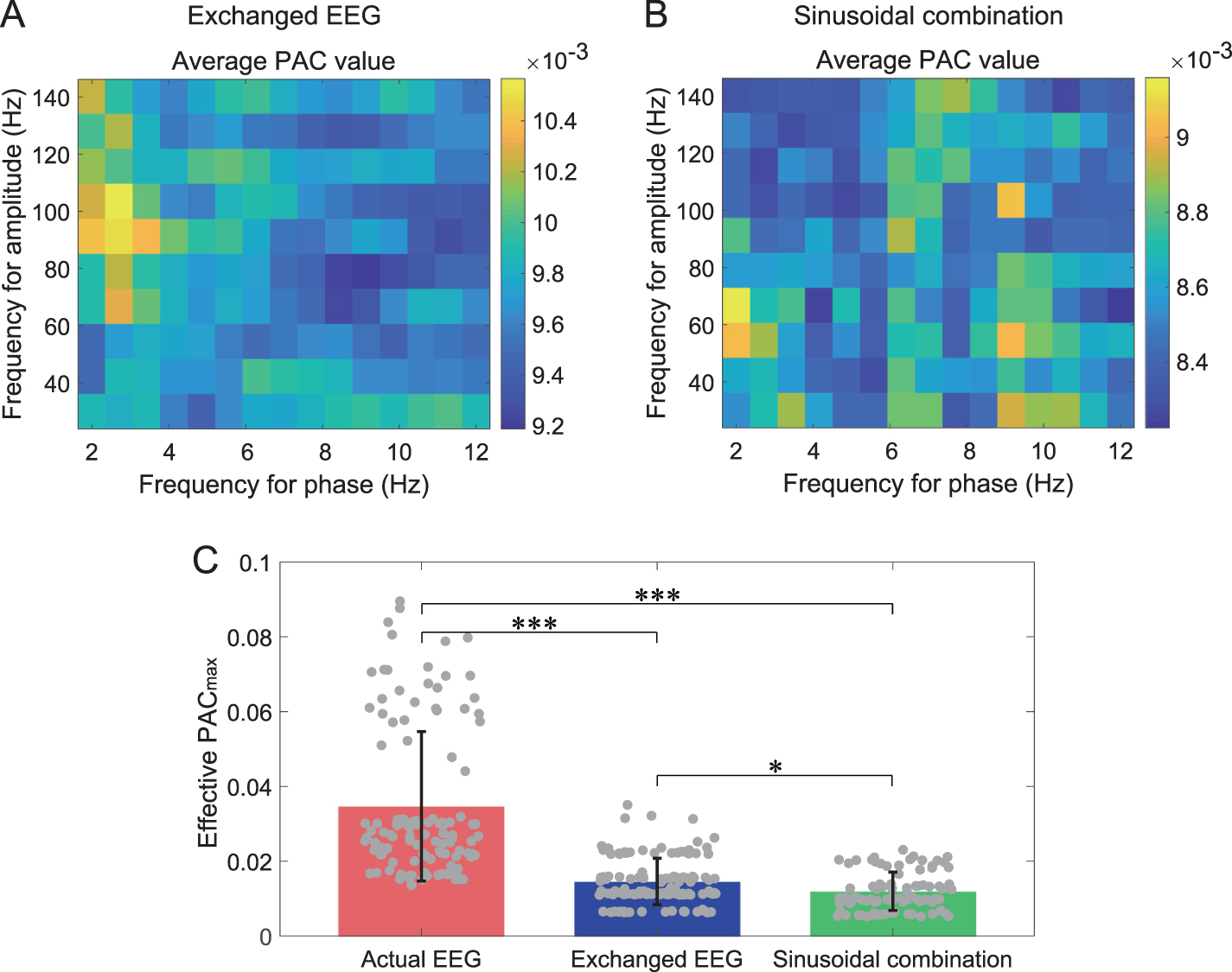
Standard image High-resolution imagePAC values calculated by the exchanged EEG and the combination of sinusoids were shown in figure 8. PAC matrixes of these two control groups showed significantly lower values than the actual PAC matrix in figure 7(C), where even the upper limits for numerical ranges in figures 8(A) and (B) were less than the lower limit in figure 7(C). The PAC matrix for the exchanged EEG showed a plausible center with relatively high values at about 2–3 Hz for the phase and 80–110 Hz for the amplitude (figure 8(A)). Still, the PAC matrix for sinusoidal combination could not show significant centralized areas for coupling (figure 8(B)). Regarding the PAC (figure 8(C)), the actual PAC
 (0.035 ± 0.02, mean ± std) was significantly higher than PAC
 values resulting from the exchanged EEG and sinusoidal combination (p
 0.001, Kruskal–Wallis test), and the values of exchanged EEG (0.015 ± 0.01) was also higher than values of sinusoidal combination (0.012 ± 0.01) (p
 0.05). Therefore, compared with the two control groups, the actual PAC values were further validated.

Figure 8. Comparisons among PAC values calculated using the actual EEG, exchanged EEG, and combination of sinusoids. (A) shows the mean of 119 surrogate PAC matrixes calculated using exchanged EEG. (B) shows the mean of 90 surrogate PAC matrixes calculated using the combination of sinusoids. The upper limits for numerical ranges in (A) and (B) were less than the lower limit for the numerical range in figure 7(C). (C) compares the PAC values calculated by the three types of signals (***p
 0.001, *p
 0.05), where the grey dots indicate the channel pairs and the error bar depicts the standard deviation.
Download figure:
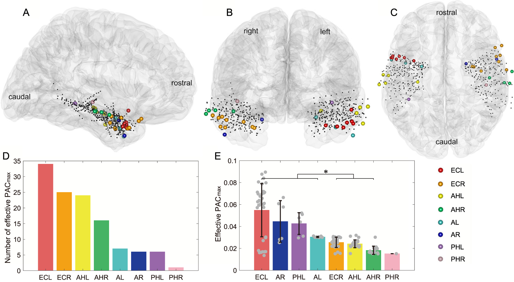
Standard image High-resolution imageAdditionally, we also identified the brain regions that contained the most effective channel pairs. Figure 9 presents the 3D locations and anatomical labels of these identified iEEG channels. Across brain regions carrying effective channel pairs, the left entorhinal cortex (ECL) produced the largest number of effective PAC values (n = 34), accounting for 29% of the total (figure 9(D)). Moreover, ECL also achieved the highest PAC
 value on average among all identified brain regions, with a value of 0.055 ± 0.024 (mean ± std, figure 9(E)). Statistical analysis showed that PAC values of ECL, bilateral amygdalas, and the left hippocampal body were significantly higher than the ones of bilateral hippocampal heads and the right entorhinal cortex (figure 9(E), p
 0.05, Wilcoxon rank sum tests).
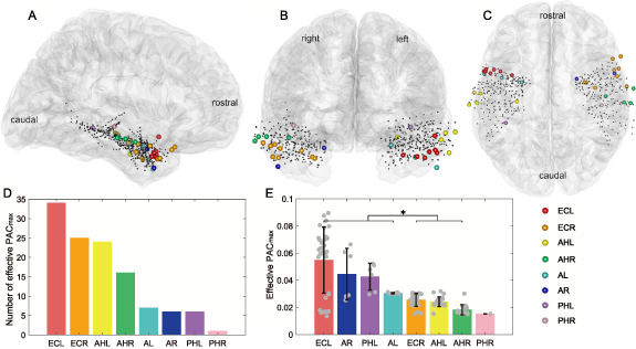
Figure 9. Distribution of iEEG channels contributing to effective PAC . (A), (B), and (C) show the standard MNI brain modal and iEEG channels in a sagittal, coronal, and transverse view, respectively. Channels belonging to different regions are marked with different colors, and abbreviations are the same as the ones above. (D) shows the number of effective PAC
 values generated by each brain region. (E) shows the average PAC
 of each region, where error bars depict the standard deviation of the values and the grey dots depict the samples.
Download figure:
Standard image High-resolution image3.3. Comparison among task periods
The average PAC matrixes across all effective channel pairs for the encoding, maintenance, and retrieval periods were shown in figures 10(A), (B), and (C) respectively. Results showed that, similarly to the matrix in figure 7(C), the maximums for all three average PAC matrixes centered uniformly at the range of 2–4 Hz for phase and 60–80 Hz for amplitude, but with different maximal levels for three task periods. The values for the retrieval period were higher than those of the other two periods. Then, for each period, when extracting the PAC value from the PAC matrix of each effective channel pair, the results suggested that the retrieval period obtained the highest PAC
 (0.087 ± 0.038, mean ± std) among the three periods, which was significantly higher than PAC
 for the encoding (0.075 ± 0.023) and maintenance (0.075 ± 0.026) periods (p = 0.02, Kruskal–Wallis test, figure 10(D).

Figure 10. PAC values of three periods in the working memory task. (A), (B), and (C) show the average PAC matrixes across all effective channel pairs for encoding, maintenance, and retrieval periods, respectively. (D) compares the PAC values extracted from the PAC matrixes among the three periods (*, p
 0.05), where the error bar depicts the standard deviation of the period, and each red dot indicates the value of an effective channel pair.
Download figure:
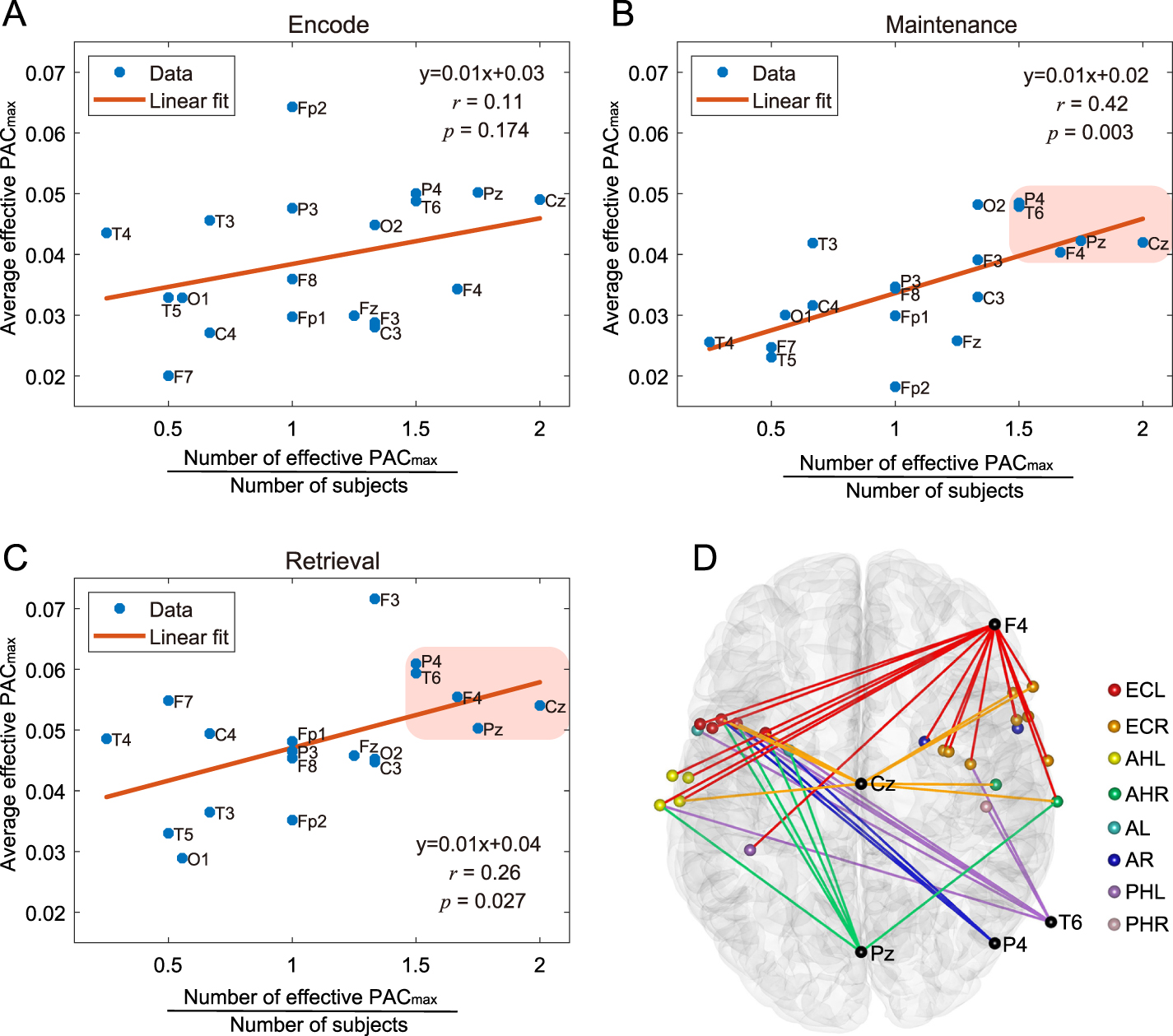
Standard image High-resolution imageFurthermore, to reveal which scalp electrodes coupled most significantly with iEEG signals during the task, we investigated the contribution to PAC of each scalp electrode for all threes periods separately (figures 11(A)–(C)). By collaboratively analyzing the number of effective PAC
 and average effective PAC
 value that related to each scalp electrode, we found that in the maintenance and retrieval periods, there was a linear positive correlation between the average effective PAC
 value and the subject-averaged number of effective PAC
 (figures 11(B) and (C)). The correlation coefficient of the maintenance and retrieval periods were 0.42 (p = 0.003) and 0.26 (p = 0.027), respectively. Among all electrodes, five electrodes (Cz, Pz, F4, P4 and T6) were closer to the upper endpoint of the regression line (figures 11(B) and (C)), suggesting that they participated in the coupling with iEEG channels more deeply than other scalp electrodes. Moreover, the connections between these scalp electrodes and the iEEG channels were widely distributed (figure 11(D)).
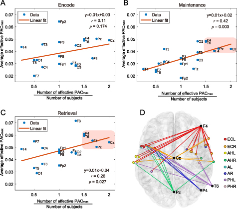
Figure 11. Scalp electrodes' contribution to PAC values. In sub-figures of (A)–(C), the horizontal ordinate indicates the number of effective PAC
 values corresponding to the scalp electrode, divided by the number of subjects that had the electrode. The vertical ordinate indicates the average effective PAC
 value generated by the scalp electrode. In (B) and (C), five electrodes (Cz, Pz, F4, P4 and T6) are closer to the upper endpoint of the regression line than other electrodes, which are highlighted by the pink area, and their connections with iEEG channels are shown in sub-figure (D) with different colors. Each connection denotes an EEG-iEEG pair generating the effective PAC
 , where scalp electrodes are highlighted with black and iEEG channels are marked with the same colors as figure 9.
Download figure:
Standard image High-resolution image3.4. Comparison among memory loads
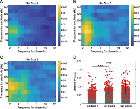
Then, we also investigated the possible difference in PAC values of the retrieval period among the three types of set size (![$n = [4,6,8]$](https://content.cld.iop.org/journals/1741-2552/19/2/026043/revision1/jneac63e9ieqn61.gif) , section 2.7). The PAC matrixes averaged across all effective channel pairs for three set sizes were shown in figures 12(A)–(C) separately. The results suggested that different set sizes induced different degrees of PAC. In detail, at about 2–4 Hz for phase and 60–80 Hz for amplitude, the set size 6 and 8 obtained higher PAC values than set size 4. Further, analysis for the PAC
, section 2.7). The PAC matrixes averaged across all effective channel pairs for three set sizes were shown in figures 12(A)–(C) separately. The results suggested that different set sizes induced different degrees of PAC. In detail, at about 2–4 Hz for phase and 60–80 Hz for amplitude, the set size 6 and 8 obtained higher PAC values than set size 4. Further, analysis for the PAC indicated that set size 6 and 8 had an average PAC
 of 0.095 ± 0.038 (mean ± std) and 0.094 ± 0.039, respectively, and there was no significant difference between these two groups (p = 0.89, Kruskal–Wallis test). In contrast, the PAC
 of set size 4 was 0.077 ± 0.034, which was significantly lower than the ones of the above two set sizes (figure 12(D), p
 0.001, Kruskal–Wallis test).
Figure 12. PAC values of three types of memory load under the retrieval period. (A), (B), and (C) show the average PAC matrixes across all effective channel pairs for set size 4, 6, and 8, respectively. (D) compares the PAC values extracted from the PAC matrixes among the three set sizes (***, p
 0.001), where the error bar depicts the standard deviation of the set size, and each red dot indicates the value of an effective channel pair.
Download figure:
Standard image High-resolution image
4. Discussion
In this study, we investigated for the first time whether the amplitude of iEEG high-gamma components is associated with the phase of low-frequency components in scalp EEG. After proving the existence of the above PAC during a working memory task, we aimed to answer a series of relevant critical questions: (a) which two frequency ranges could generate the coupling; (b) which intracerebral structures and scalp electrodes resulted in the most significant coupling; (c) whether PAC values were influenced by different task periods and memory loads.
4.1. Interpretations of iEEG frequency bands and PAC
PAC provides effective integration of activities across different spatial and temporal scales [36], therefore, PAC has developed as an indicator to describe the functional interaction between deep brain and scalp regions. For example, Damborská et al have demonstrated the coupling between the delta/theta phase of iEEG and amplitude of higher frequency bins of scalp EEG [24]. In contrast, the current study proved the existence of PAC phenomenon between the low-frequency band of scalp EEG and the high-gamma band of iEEG.
Regarding the low-frequency band of scalp EEG, we found the frequency range that generated the PAC centered at 2–4 Hz in general, and this range could be up to around 6 Hz in particular channel pairs (figure 6, subject 6). Hence, the phase frequency for PAC stretched over the delta and theta bands in general. Unlike the high-gamma activities, which is a reliable indicator of local neural population-level activities [37–39], low-frequency oscillatory activities from the delta band to the alpha band are inversely related to the number of synchronously active neurons in a neural network [40]. Therefore, oscillatory activities in delta and theta bands are considered as carrier frequencies for communication between distant brain regions [5, 41, 42], which might reflect functional connectivity among large-scale brain regions [43–46].
Because of the above physiological interpretations, PAC might serve as an information transmission mechanism, where low-frequency oscillations of large-scale intracranial networks regulate the high-frequency local processing, thus integrating functional organizations across multiple spatiotemporal scales [36]. This important idea could be reflected in this study. More specifically, the intracerebral regions generating PAC in the current study might belong to a distributed network processing the memory task [47, 48], where high-gamma activities of local nodes are modulated by intracranial delta/theta information flows. This hypothesis is in accordance with previous iEEG studies proving that high-gamma amplitude was significantly modulated by delta or theta phase [49, 50]. Meanwhile, due to the low-pass-filter effect of the skull [20] and the volume conduction [9], the intracranial delta/theta network might generate an imitation with deflections and noises at the scalp. In this view, EEG signals recorded at the scalp electrodes can be regarded as incomplete descriptions of the imitative network [51]. Therefore, the above views may explain the existence of PAC between the low-frequency band of scalp EEG and the high-gamma band of iEEG in this study. Additionally, the PAC validation by control groups derived another interesting phenomenon: there was plausible PAC between cross-subject channel pairs when we implemented the PAC calculation using the exchanged EEG (figure 8(A)). The PAC resulting from the exchanged EEG was significantly higher than the level resulting from sinusoidal combination (p
 0.05, figure 8(C)), even though the exchanged EEG resulted in much lower PAC than the actual PAC. One possible explanation for this cross-subject PAC might be that the scalp EEG features have a modest degree of transferability across subjects [52, 53], so slight similarities among scalp EEG signals of different subjects might result in slighter similarities between the actual PAC and the PAC calculated by exchanged EEG.
4.2. Region participation in the working memory task
From the view of intracranial-extracranial functional connectivity, the emerging combination of iEEG and scalp EEG could provide a new indicator for evaluating region participation in the memory task. PAC values in the current study showed significant differences among task periods and memory loads, suggesting that the corresponding intracerebral structures' functional linkages with scalp areas were indeed influenced by the memory load. Similarly, the phase-phase coupling analysis, as another functional connectivity indicator, has also been adopted to identify the hippocampal linkages with scalp areas, and the phase-locking value was also load-sensitive during the working memory task [26].
Regarding the proposed PAC , bilateral entorhinal cortexes and hippocampal heads generated the most effective PAC
 values (99 out of 119). Though bilateral amygdalas and the left hippocampal body contributed relatively few numbers of effective PAC
 values, the average effective PAC
 values in these regions were at a relatively high level. As far as both the number and the level of effective PAC
 values, ECL achieved the best performance among all regions, suggesting its vital involvement in subcortico-cortical interactions. The role of these regions in the verbal working memory task could be identified to a certain extent by previous fMRI studies. For example, the entorhinal cortex, as a part of the major pathway modulating input to the hippocampus, was related to the activations of frontal regions during memory retrieval [48]. Additionally, hippocampal regions could be more active during retrieval than maintenance [54], and hippocampal interactions with cortical areas were vital to successful memory formation [47]. Amygdala activities were even linked to the response speed during working memory [55]. Besides fMRI, iEEG recordings in this study could explore these brain regions' local activations during the working memory task from a new perspective. Additionally, the high-gamma activity of iEEG displayed the evolution of local activation (figure 5), and this temporal information could not be detected by fMRI measurement. Most importantly, we showed that five scalp areas (Cz, Pz, F4, P4, and T6) resulted in more significant PAC
 values than other scalp electrodes (figure 11). Four out of these selected scalp electrodes existed among four subjects in the whole dataset, whereas many other electrodes existed among nine subjects (figure 1). Therefore, the superiority of these selected electrodes was not caused by selection bias. These findings might suggest a large-scale frontal-parietal-temporal scalp network reflecting partial intracerebral activities during the memory task. Interestingly, all selected scalp locations were at the midline or right hemisphere. This dominance of the right hemisphere might be in accordance with fMRI studies, which demonstrated that increasing memory load was associated with right hemisphere dominance [56]. Previous scalp EEG studies have also suggested potential roles of parietal, frontal, and temporal areas in memory tasks [57–59], and we enhanced the significance and credibility of these scalp EEG findings by setting intracranial activations as the criterion.
4.3. Implications and future work
Potent correlation between the envelopes of iEEG and scalp EEG components is the physiological basis of mapping scalp EEG to iEEG within the low-frequency band [9]. Regarding the high-frequency components, there indeed exist studies that find similarities between high-gamma (60–85 Hz) responses extracted from iEEG and scalp EEG [60]. This direct measurement of high-gamma responses from scalp EEG depends on several optimized configurations, including high amplification, meticulous signal processing, and a paradigm with higher inducibility of high-gamma activities [60]. Additionally, novel deep convolution neural networks can also extract high-gamma activities (71–91 Hz) from scalp EEG [61]. However, one unfailing concern has been that subtle high-gamma activities in scalp EEG are likely to be obscured by electrical artifacts and scalp electromyography [62, 63], and only a small fraction of high-frequency source power, as recorded by iEEG, can be recorded by scalp EEG [20]. In another way, the PAC in this study provided the physiological basis for estimating the amplitude of iEEG high-gamma band based on the phase of low-frequency scalp EEG. Moreover, results might herald more significant intracranial representations at Cz, Pz, F4, P4 and T6 than other scalp locations under the current task (figure 11). These explorations on the relationship between intracranial signals and their scalp EEG correlates are crucial to developing and validating potential surrogates for invasive recordings in the future [64]. Therefore, based on the observed PAC, we would also verify the possibility of mapping scalp EEG signals to features derived from iEEG high-frequency components.
There were also some limitations in this work. Due to limited computing power, the current work only calculated general PAC values of different task periods instead of the temporal evolution of PAC during the whole experiment process. However, the temporal evolution of PAC is of great importance for a deeper understanding of neural information transmission. To our knowledge, the emerging PAC calculation approach based on local mutual information is suitable for estimating the temporal evolution of PAC [21], but this approach is computationally expensive, especially when hundreds of surrogates have to be generated to evaluate the statistical significance of PAC values [33]. In future work, we would calculate the PAC temporal evolution based on the local mutual information approach when computing equipment with high performance is available.
5. Conclusion
Simultaneous iEEG and scalp EEG recordings are crucial to investigations on the information flow from intracerebral regions to the scalp. We proposed a PAC analysis strategy to valid the non-invasive representation of iEEG features derived from high-frequency bands. The PAC phenomenon has been proven widespread and discriminable among different task periods and memory loads. The findings of this study broaden our understanding of neural information transmission, and provide essential clues for future estimations of iEEG via scalp EEG.
Data availability statement
The data that support the findings of this study are openly available at the following URL/DOI: 10.1038/s41597-020-0364-3.
Acknowledgments
We would like to thank Boran E, Fedele T, Steiner A, Hilfiker P, Stieglitz L, Grunwald T, and Sarnthein J for presenting the precious dataset [25].
This work is supported in part by the China National Key R&D Program (Grant No. 2018YFB1307200), and the National Natural Science Foundation of China (Grant Nos. 91948302, 52105030).